Why measure theory: the limits of the Riemann integral

In MATH-341 the Riemann integral was the workhorse: we integrated continuous functions on closed intervals, swapped limits and integrals under uniform convergence, and proved the fundamental theorem of calculus. This course replaces that integral with a more powerful one, built by Henri Lebesgue in his 1902 thesis, and develops the theory of measure on which it rests. Before building anything, this lesson explains why the replacement is needed. We look at three places where the Riemann integral fails: it cannot integrate many functions that arise as limits of perfectly good functions, its convergence theorems need hypotheses that are too strong for analysis and probability, and the space of Riemann integrable functions is not complete under the natural distance. Each failure points to the same remedy: measure the size of sets in the range of a function's values, not just intervals in its domain.

Riemann sums slice the domain

Recall the definition. For a bounded function \(f\) on \([a, b]\) and a partition \(P = \{a = x_0 < x_1 < \cdots < x_n = b\}\), the upper and lower sums are \[U(f, P) = \sum_{i=1}^{n} M_i (x_i - x_{i-1}), \qquad L(f, P) = \sum_{i=1}^{n} m_i (x_i - x_{i-1}),\] where \(M_i\) and \(m_i\) are the supremum and infimum of \(f\) on \([x_{i-1}, x_i]\). The function is Riemann integrable when \(\sup_P L(f, P) = \inf_P U(f, P)\), and the common value is \(\int_a^b f\). The partition chops the domain into intervals, and on each interval the function is replaced by a constant. This works well when \(f\) varies little across short intervals, which is exactly what continuity provides. It works badly for functions that oscillate wildly on every interval, however short.

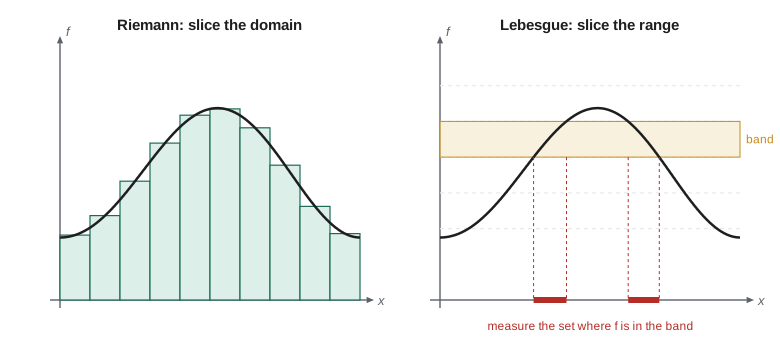
Lebesgue described the difference with an analogy that is worth repeating. Suppose you must count a pile of coins. The Riemann method takes the coins in the order they come and adds their values one by one. The Lebesgue method first sorts the coins by denomination, counts how many of each kind there are, and multiplies. Both give the same total for a finite pile, but the second method does not care how the coins are arranged, and it extends to situations where the first one breaks down. For a function, sorting by denomination means grouping points of the domain by the value of \(f\): for each horizontal band \(y_{k-1} \le f < y_k\), we ask how large the set \(\{x : y_{k-1} \le f(x) < y_k\}\) is, and form \[\sum_k y_{k-1} \, \mu\big(\{x : y_{k-1} \le f(x) < y_k\}\big).\] Here \(\mu\) is a way to measure the size of sets that may be far more complicated than intervals. Making \(\mu\) precise is the main work of the first four lessons.

Failure one: limits of integrable functions

Enumerate the rational numbers in \([0, 1]\) as \(q_1, q_2, q_3, \ldots\) and let \(f_n\) be the indicator function of the finite set \(\{q_1, \ldots, q_n\}\): \(f_n(x) = 1\) if \(x\) is one of the first \(n\) rationals and \(0\) otherwise. Each \(f_n\) is zero except at finitely many points, so it is Riemann integrable with \(\int_0^1 f_n = 0\). The sequence increases, \(0 \le f_1 \le f_2 \le \cdots \le 1\), and converges at every point to the Dirichlet function \[D(x) = \begin{cases} 1 & x \in \mathbb{Q}, \\ 0 & x \notin \mathbb{Q}. \end{cases}\] Every subinterval of a partition contains both rationals and irrationals, so \(M_i = 1\) and \(m_i = 0\) for all \(i\). Hence \(U(D, P) = 1\) and \(L(D, P) = 0\) for every partition, and \(D\) is not Riemann integrable. A bounded, monotone sequence of integrable functions with integrals all equal to zero converges to a function that the theory cannot integrate at all.

This is not a pathology that can be ignored. Limits are the lifeblood of analysis: we define functions by series, solve differential equations by successive approximation, and represent signals by Fourier series. A theory of integration in which a monotone limit of integrable functions can fail to be integrable forces us to verify integrability at every step. The Lebesgue integral will assign \(\int D = 0\), because the rationals form a set of measure zero, and the monotone convergence theorem of lesson 6 will guarantee that \(\int f_n \to \int D\) without any extra hypothesis.

# Riemann sums of the Dirichlet function depend entirely on the sample points.
from fractions import Fraction
import math

def D(x):
    """1 on rationals, 0 on irrationals; x is a Fraction or a float tagged irrational."""
    return 1 if isinstance(x, Fraction) else 0

n = 1000
left_rational = sum(D(Fraction(i, n)) for i in range(n)) / n
# shift every sample point by an irrational amount that keeps it inside the subinterval
irr_points = [(i + math.sqrt(2) - 1) / n for i in range(n)]
left_irrational = sum(D(x) for x in irr_points) / n
print("Riemann sum with rational sample points:  ", left_rational)
print("Riemann sum with irrational sample points:", left_irrational)
print("Upper sum is 1 and lower sum is 0 for every partition, so no limit exists.")

Riemann sum with rational sample points:   1.0
Riemann sum with irrational sample points: 0.0
Upper sum is 1 and lower sum is 0 for every partition, so no limit exists.

Failure two: convergence theorems with heavy hypotheses

In MATH-341 we proved that if \(f_n \to f\) uniformly on \([a, b]\) and each \(f_n\) is Riemann integrable, then \(f\) is Riemann integrable and \(\int f_n \to \int f\). Uniform convergence is a strong requirement. Many sequences of interest converge pointwise but not uniformly, and for them we want a usable criterion. For example, \(f_n(x) = x^n\) on \([0, 1]\) converges pointwise to the function that is \(0\) on \([0, 1)\) and \(1\) at \(1\). The convergence is not uniform, since \(\sup_{[0,1)} x^n = 1\) for every \(n\), yet \(\int_0^1 x^n = \frac{1}{n+1} \to 0\), the integral of the limit. Something other than uniformity makes this work: the functions are bounded by the integrable function \(1\). Lebesgue's dominated convergence theorem, proved in lesson 7, says exactly that pointwise convergence together with a single integrable bound is enough.

The hypothesis cannot simply be dropped. On \([0, 1]\) let \(g_n = n \cdot \mathbf{1}_{(0, 1/n)}\), a tall thin rectangle of height \(n\) and width \(\frac{1}{n}\). Then \(g_n(x) \to 0\) for every \(x\), but \(\int_0^1 g_n = 1\) for every \(n\). The mass of the rectangles does not disappear; it escapes into a single point. Similarly \(h_n = \mathbf{1}_{[n, n+1]}\) on the real line converges to zero pointwise while \(\int h_n = 1\): the mass escapes to infinity. A good convergence theorem must explain both examples, and the dominated convergence theorem does: no single integrable function lies above all the \(g_n\) or all the \(h_n\).

Failure three: an incomplete space

On the space of continuous functions on \([0, 1]\), define the distance \(d_1(f, g) = \int_0^1 |f - g|\). In MATH-341 we saw that this metric space is not complete: a sequence of continuous functions can be Cauchy in \(d_1\) while its natural limit is discontinuous. Enlarging the space to all Riemann integrable functions does not fix the problem. Here is a concrete sequence. Let \(F_n\) be the indicator function of the union of the open intervals of length \(4^{-k}\) removed at the \(k\)th step of a fat Cantor set construction, for \(k \le n\). Each \(F_n\) is a step function with finitely many jumps, hence Riemann integrable, and \(d_1(F_n, F_m) = \sum_{k=n+1}^{m} 2^{k-1} 4^{-k} \to 0\). The limit is the indicator function of an open set \(U\) whose complement is a closed set of positive length with empty interior. That indicator is discontinuous at every point of the complement, a set of positive length, and by the Lebesgue criterion proved in lesson 8 it is not Riemann integrable.

Completeness matters because so much of analysis consists of constructing an object as the limit of approximations: the solution of a differential equation, the minimizer of an energy, the sum of a Fourier series. If the space of functions is not complete, Cauchy sequences may have no limit to construct. The space \(L^1\) of Lebesgue integrable functions, studied in lesson 11, is complete; this is the Riesz–Fischer theorem, and it is one of the main reasons the Lebesgue integral is the standard integral of modern analysis.

What a measure has to do

All three failures point to the need to measure the size of sets that are not finite unions of intervals: the rationals, the set where a function lies in a band, the complement of a fat Cantor set. We would like a function \(m\) defined on every subset of \(\mathbb{R}\), taking values in \([0, \infty]\), with three properties: it gives each interval its length, so \(m([a, b]) = b - a\); it is translation invariant, so \(m(E + t) = m(E)\); and it is countably additive, so that for pairwise disjoint sets \(E_1, E_2, \ldots\), \[m\Big(\bigcup_{k=1}^{\infty} E_k\Big) = \sum_{k=1}^{\infty} m(E_k).\] Countable additivity, rather than just finite additivity, is what makes limit theorems possible: it lets us compute the size of a set built by a countable process from the sizes of its pieces.

A theorem of Giuseppe Vitali from 1905, proved in lesson 4, shows that no such function exists on all subsets of the line. Using the axiom of choice, Vitali constructed a set whose translates by rationals tile \([0, 1)\) in a way that makes any value of its measure contradictory. The resolution is to give up the demand that every set be measurable. We define the measure only on a large collection of sets, a σ-algebra, which is closed under complements and countable unions and contains every set that arises in practice. The cost is a little bookkeeping: we must check that the sets and functions we use are measurable. The benefit is a theory with powerful and clean limit theorems.

The example shows something surprising about size. The rationals are dense: every interval, however small, contains infinitely many of them. Yet as a set they are negligible, with total length zero. Density is a topological notion and measure is a different one, and much of this course concerns the interplay between them. A set can be dense and of measure zero, like the rationals, or nowhere dense and of positive measure, like the fat Cantor set mentioned above.

Lebesgue sums in practice

For a continuous function the Riemann and Lebesgue constructions agree, and comparing them numerically builds intuition for the new approach. To compute a Lebesgue sum, choose levels \(0 = y_0 < y_1 < \cdots < y_N\) covering the range of \(f\), estimate the measure of each set \(\{y_{k-1} \le f < y_k\}\), and add. For a nice function on an interval, those sets are finite unions of intervals whose lengths can be found from the points where \(f\) crosses the levels. In the code below we estimate them by sampling a fine grid, which is a crude way to approximate measure, but it already shows that the Lebesgue sum approaches the same value as the Riemann sum as the levels are refined.

# Riemann (domain slicing) versus Lebesgue (range slicing) for f(x) = x * (1 - x) * 4 on [0, 1].
def f(x):
    return 4 * x * (1 - x)

exact = 2 / 3

def riemann(n):
    return sum(f((i + 0.5) / n) for i in range(n)) / n

def lebesgue(levels, grid=200000):
    # measure of {y_(k-1) <= f < y_k} estimated by the fraction of grid points in the band
    counts = [0] * levels
    for i in range(grid):
        y = f((i + 0.5) / grid)
        k = min(int(y * levels), levels - 1)
        counts[k] += 1
    # lower Lebesgue sum: band value y_(k-1) times measure of the band
    return sum((k / levels) * c / grid for k, c in enumerate(counts))

for n in (4, 16, 64):
    print(f"n = {n:3d}: Riemann midpoint {riemann(n):.6f}   lower Lebesgue {lebesgue(n):.6f}")
print("exact integral:", round(exact, 6))

n =   4: Riemann midpoint 0.687500   lower Lebesgue 0.518285
n =  16: Riemann midpoint 0.667969   lower Lebesgue 0.632332
n =  64: Riemann midpoint 0.666748   lower Lebesgue 0.658458
exact integral: 0.666667

The lower Lebesgue sum underestimates the integral by at most the band height times the total length, \(\frac{1}{N}\), because on each band \(f\) exceeds the band value \(y_{k-1}\) by less than \(\frac{1}{N}\). This simple error bound, which needs no continuity at all, is the heart of the matter. It holds for any bounded function whose band sets can be measured. In lesson 5 we will make it the basis of simple-function approximation: every nonnegative measurable function is the increasing limit of functions taking finitely many values, each on a measurable set.

Where the course goes

The plan of the course follows the logic just described. Lesson 2 sets up the abstract framework of σ-algebras and measures, which covers not only length on the line but also counting measure, probability distributions and area. Lesson 3 constructs Lebesgue measure through outer measure and Carathéodory's criterion. Lesson 4 explores the measurable sets: Borel sets, Cantor sets, and Vitali's non-measurable set. Lessons 5 to 7 build the integral and prove its three great convergence theorems: monotone convergence, Fatou's lemma and dominated convergence. Lesson 8 compares the new integral with the Riemann integral and proves Lebesgue's criterion for Riemann integrability. Lesson 9 sorts out the different ways a sequence of functions can converge. Lesson 10 builds product measures and proves the theorems of Fubini and Tonelli on iterated integrals. Lesson 11 studies the \(L^p\) spaces, and the capstone in lesson 12 connects the theory to differentiation and to probability, where Andrey Kolmogorov's 1933 axioms made measure theory the foundation of the subject.

Historically the subject grew quickly. Bernhard Riemann gave his definition of the integral in his 1854 Habilitation essay on trigonometric series, a context in which the integrability of limits was exactly the question at stake. Émile Borel introduced measure for countable unions of intervals in 1898. Lebesgue's thesis, Intégrale, longueur, aire, appeared in 1902, and within twenty years Vitali, Pierre Fatou, Guido Fubini, Leonida Tonelli, Frigyes Riesz, Ernst Fischer, Johann Radon and Constantin Carathéodory had built most of what this course covers. The abstraction to general measure spaces, essential for probability, was complete by the time of Otton Nikodym's theorem in 1930.

Throughout the course, the companion Python examples use only the standard library. They cannot compute Lebesgue measure of an arbitrary set, which is not a finite computation, but they can illustrate constructions, test inequalities numerically, and show counterexamples behaving as the theory predicts. Reading the code alongside the proofs is a good habit: a proof explains why a statement holds, and a computation shows what it looks like.