Separation of variables for the heat equation · MATH-336 Lesson 7

Separation of variables is the method Fourier invented to solve heat problems, and it remains the most important exact technique for linear PDEs on simple domains. The idea is to look for solutions that are products of a function of $x$ alone and a function of $t$ alone. The PDE then splits into two ODEs linked by a separation constant, the boundary conditions turn the spatial ODE into an eigenvalue problem, and superposition of the resulting product solutions, with coefficients from a Fourier series, matches the initial condition. This lesson carries out the method for the heat equation with Dirichlet, Neumann and mixed boundary conditions, handles nonzero boundary temperatures with a steady state, and draws out the physical meaning of the series: smoothing, exponential decay and the dominance of the slowest mode.

Product solutions

Consider the problem for a rod of length $L$ with both ends held at zero temperature:

\[u_t = \alpha u_{xx}\ \ (0 < x < L,\ t > 0), \qquad u(0, t) = u(L, t) = 0, \qquad u(x, 0) = f(x)\]

Try $u(x, t) = X(x)T(t)$. Substituting gives $XT' = \alpha X''T$, and dividing by $\alpha XT$,

\[\frac{T'(t)}{\alpha T(t)} = \frac{X''(x)}{X(x)}\]

The left side depends only on $t$ and the right only on $x$. If a function of $t$ equals a function of $x$ for all $x$ and $t$, both must equal the same constant, which we call $-\lambda$. So $X'' + \lambda X = 0$ and $T' = -\lambda\alpha T$. The boundary conditions apply to $X$: from $X(0)T(t) = 0$ for all $t$ and $T$ not identically zero, $X(0) = 0$, and likewise $X(L) = 0$. The initial condition will be handled at the end by superposition.

The eigenvalue problem

We need the values of $\lambda$ for which $X'' + \lambda X = 0$, $X(0) = X(L) = 0$ has a solution other than $X \equiv 0$. Such $\lambda$ are eigenvalues and the corresponding $X$ eigenfunctions. Consider the three cases.

If $\lambda < 0$, write $\lambda = -\mu^2$ with $\mu > 0$. Then $X = A\cosh\mu x + B\sinh\mu x$; $X(0) = 0$ gives $A = 0$ and $X(L) = B\sinh\mu L = 0$ gives $B = 0$, since $\sinh\mu L > 0$. No eigenvalue. If $\lambda = 0$, $X = A + Bx$ and both conditions force $A = B = 0$. No eigenvalue. If $\lambda = \mu^2 > 0$, $X = A\cos\mu x + B\sin\mu x$; $X(0) = 0$ gives $A = 0$, and $X(L) = B\sin\mu L = 0$ with $B \ne 0$ requires $\sin\mu L = 0$, so $\mu L = n\pi$. The eigenvalues and eigenfunctions are

\[\lambda_n = \Big(\frac{n\pi}{L}\Big)^2, \qquad X_n(x) = \sin\frac{n\pi x}{L}, \qquad n = 1, 2, 3, \ldots\]

A neat argument rules out non-positive eigenvalues in one step. Multiply $X'' + \lambda X = 0$ by $X$ and integrate by parts: $\lambda\int_0^L X^2\,dx = -\int_0^L XX''\,dx = -[XX']_0^L + \int_0^L (X')^2\,dx = \int_0^L (X')^2\,dx$. So $\lambda \ge 0$, with $\lambda = 0$ only if $X$ is constant, which the Dirichlet conditions forbid. This energy identity is the same idea as the uniqueness proof of lesson 1.

With $\lambda = \lambda_n$, the time equation gives $T_n(t) = e^{-\alpha\lambda_n t}$, so the product solutions are $e^{-\alpha(n\pi/L)^2t}\sin(n\pi x/L)$. Each one is a sine-shaped temperature profile that keeps its shape and decays exponentially, with decay rate proportional to the square of its wavenumber.

Superposition and the Fourier sine series

Since the equation and boundary conditions are linear and homogeneous, any sum of product solutions is a solution:

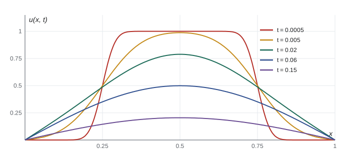
\[u(x, t) = \sum_{n=1}^\infty b_n\,e^{-\alpha(n\pi/L)^2t}\sin\frac{n\pi x}{L}, \qquad b_n = \frac2L\int_0^L f(x)\sin\frac{n\pi x}{L}\,dx\]

At $t = 0$ the series is the Fourier sine series of $f$, so choosing the $b_n$ as the sine coefficients satisfies the initial condition. This is where lesson 5 pays off: the Dirichlet boundary conditions produced sine eigenfunctions, and the odd extension of $f$ produces exactly the matching series. For $t > 0$ the factors $e^{-\alpha(n\pi/L)^2t}$ decay so fast that the series converges absolutely and can be differentiated term by term as often as we like. Even if $f$ has jumps, $u$ is infinitely differentiable for every $t > 0$: the heat equation smooths instantly. A uniqueness argument (lesson 1) shows this is the only solution.

Worked problem

A hot block in a cold rod

Solve the problem with $L = 1$, $\alpha = 1$ and $f(x) = 1$ for $\frac14 < x < \frac34$, zero elsewhere.

Show solution

$b_n = 2\int_{1/4}^{3/4}\sin n\pi x\,dx = \frac{2}{n\pi}\big(\cos\frac{n\pi}{4} - \cos\frac{3n\pi}{4}\big)$.
For $n = 1$: $b_1 = \frac{2}{\pi}\cdot\sqrt2 \approx 0.900$. For $n = 2$: $\cos\frac\pi2 - \cos\frac{3\pi}{2} = 0$, so $b_2 = 0$, and by symmetry every even coefficient vanishes. For $n = 3$: $b_3 = \frac{2}{3\pi}(-\sqrt2) \approx -0.300$.
The solution is $u = \sum b_n e^{-n^2\pi^2t}\sin n\pi x$. By $t = 0.1$ the factor for $n = 3$ is $e^{-8.9} \approx 1.4 \times 10^{-4}$, so $u \approx 0.900\,e^{-\pi^2t}\sin\pi x$.

Answer: The block rounds off within a few thousandths of a time unit and then decays as a single sine arch at rate $\pi^2$. The total heat $\int_0^1 u\,dx$ decreases from 0.5 because heat leaks out through the cold ends.

$Temperature profiles on 0 to 1 at five times. At t equals 0.0005 the profile is a nearly square block from 0.25 to 0.75 at height 1 with slight ripples. At t equals 0.005 the corners are rounded. By t equals 0.02 it is a smooth hump of height about 0.8; at t equals 0.06 a lower sine-like arch; at t equals 0.15 a low arch of height about 0.2.$

Series solution for a block of heat in a rod with ice-cold ends ($\alpha = 1$): corners vanish almost instantly, and after $t \approx 0.05$ the profile is essentially the first mode $\sin\pi x$ decaying like $e^{-\pi^2t}$

Other boundary conditions

Insulated ends, $u_x(0, t) = u_x(L, t) = 0$, lead to $X'' + \lambda X = 0$, $X'(0) = X'(L) = 0$. Now $\lambda = 0$ is an eigenvalue with constant eigenfunction, and the full set is $\lambda_n = (n\pi/L)^2$, $X_n = \cos(n\pi x/L)$ for $n = 0, 1, 2, \ldots$. The solution is a cosine series,

\[u(x, t) = \frac{a_0}{2} + \sum_{n=1}^\infty a_n\,e^{-\alpha(n\pi/L)^2t}\cos\frac{n\pi x}{L}, \qquad a_n = \frac2L\int_0^L f(x)\cos\frac{n\pi x}{L}\,dx\]

As $t \to \infty$, $u \to a_0/2$, the average initial temperature. This is physically right: an insulated rod loses no heat, so its total heat content is conserved, and it ends at a uniform temperature with the same content.

Mixed conditions, such as the copper rod of lesson 1 with $u(0, t) = 0$ and $u_x(L, t) = 0$, give $X(0) = 0$, $X'(L) = 0$. Then $X = \sin\mu x$ with $\cos\mu L = 0$, so $\mu_n = (2n - 1)\pi/(2L)$: only the odd quarter-wave harmonics appear. For a constant initial temperature $T_0$,

\[u(x, t) = \frac{4T_0}{\pi}\sum_{n=1}^\infty \frac{1}{2n - 1}\,e^{-\alpha\mu_n^2t}\sin\mu_n x, \qquad \mu_n = \frac{(2n - 1)\pi}{2L}\]

The slowest decay rate is $\alpha\pi^2/(4L^2)$, four times slower than for a rod with both ends cold, because heat must travel the whole length to escape. For the 50 cm copper rod at 20 °C, $\alpha\mu_1^2 = 1.1 \times 10^{-4}\cdot\pi^2/1 \approx 1.09 \times 10^{-3}$ per second, so the insulated end cools with a time constant of about 15 minutes.

Nonzero boundary temperatures

If the ends are held at fixed temperatures $u(0, t) = T_1$ and $u(L, t) = T_2$, the boundary conditions are not homogeneous and product solutions cannot satisfy them. The remedy is to subtract the steady state. The equilibrium temperature $v(x)$ satisfies $v'' = 0$, $v(0) = T_1$, $v(L) = T_2$, so $v = T_1 + (T_2 - T_1)x/L$. The transient $w = u - v$ then satisfies the heat equation with zero boundary values and initial condition $f - v$, which separation solves. The full solution is

\[u(x, t) = T_1 + (T_2 - T_1)\frac{x}{L} + \sum_{n=1}^\infty c_n\,e^{-\alpha(n\pi/L)^2t}\sin\frac{n\pi x}{L}, \qquad c_n = \frac2L\int_0^L (f - v)\sin\frac{n\pi x}{L}\,dx\]

The same trick works for steady sources: subtract the solution of $\alpha v'' = -Q/(\rho c)$ with the given boundary values. Time-dependent boundary data or sources need an extension, the method of eigenfunction expansion, in which the coefficients $c_n(t)$ satisfy ODEs driven by the projected forcing. A Robin condition $u_x(L, t) + hu(L, t) = 0$ leads to the transcendental eigenvalue equation $\tan\mu L = -\mu/h$, whose roots must be found numerically; the eigenfunctions $\sin\mu_nx$ are still orthogonal. All these problems are instances of Sturm–Liouville theory, developed by Charles Sturm and Joseph Liouville in the 1830s, which guarantees real eigenvalues, orthogonal eigenfunctions and convergent expansions for the general equation $(pX')' + (\lambda w - q)X = 0$.

What the series tells us

Three facts make the heat series one of the most informative formulas in applied mathematics. First, the modes decay at rates $\alpha(n\pi/L)^2$, so after a time comparable to $L^2/(\alpha\pi^2)$ every mode but the first is negligible; the late-time profile is $b_1e^{-\alpha\pi^2t/L^2}\sin(\pi x/L)$ regardless of how the rod started. Second, the series shows the maximum principle at work: the solution never exceeds the larger of its initial and boundary maxima. Third, running time backward multiplies mode $n$ by $e^{+\alpha(n\pi/L)^2|t|}$, so tiny high-frequency errors in a measured final temperature explode; reconstructing the past of a diffusion process is ill posed, exactly as Hadamard warned.

Evaluating the series

The program evaluates the block solution and checks it in several ways: the initial partial sums approximate the block, the boundary values are zero, the PDE residual is small, the total heat matches a separate formula, and the late profile matches the first mode. It also computes how long the insulated end of the copper rod takes to reach 1 °C.

Evaluating the heat series: coefficients, smoothing, decay to the first mode, total heat, and the cooling time of an insulated rod end

import math

L, alpha = 1.0, 1.0
def b(n):
    return 2 / (n * math.pi) * (math.cos(n * math.pi / 4) - math.cos(3 * n * math.pi / 4))
def u(x, t, N=400):
    return sum(b(n) * math.exp(-alpha * (n * math.pi / L) ** 2 * t) * math.sin(n * math.pi * x / L) for n in range(1, N + 1))

print("b_1..b_7:", " ".join(f"{b(n) + 0.0:+.4f}" for n in range(1, 8)))
print("t = 0 partial sums:", [round(u(x, 0.0), 3) for x in (0.1, 0.3, 0.5, 0.7, 0.9)])
for t in (0.001, 0.01, 0.05, 0.1):
    h, k = 1e-3, 1e-6
    x = 0.4
    res = (u(x, t + k) - u(x, t - k)) / (2 * k) - alpha * (u(x + h, t) - 2 * u(x, t) + u(x - h, t)) / h ** 2
    heat = sum(b(n) * math.exp(-(n * math.pi) ** 2 * t) * 2 / (n * math.pi) for n in range(1, 400, 2))
    one_mode = b(1) * math.exp(-math.pi ** 2 * t)
    print(f"t = {t:5.3f}: u(0.5) = {u(0.5, t):.5f}, first mode only {one_mode:.5f}, "
          f"total heat {heat:.5f}, PDE residual {res:+.1e}, u(0) = {u(0.0, t):.1e}")

# copper rod: u(0,t) = 0, u_x(L,t) = 0, starts at 20 C; when does x = L reach 1 C?
a, Lr, T0 = 1.1e-4, 0.5, 20.0
mu = lambda n: (2 * n - 1) * math.pi / (2 * Lr)
end = lambda t: 4 * T0 / math.pi * sum((-1) ** (n + 1) / (2 * n - 1) * math.exp(-a * mu(n) ** 2 * t) for n in range(1, 200))
lo, hi = 0.0, 1e5
for _ in range(60):
    mid = (lo + hi) / 2
    lo, hi = (mid, hi) if end(mid) > 1.0 else (lo, mid)
print(f"insulated end: {end(0.0):.2f} C at t = 0, 1 C after {hi / 60:.1f} minutes")
print(f"slowest time constant 1/(alpha mu_1^2) = {1 / (a * mu(1) ** 2) / 60:.1f} minutes")

Output

b_1..b_7: +0.9003 +0.0000 -0.3001 +0.0000 -0.1801 -0.0000 +0.1286
t = 0 partial sums: [0.001, 0.994, 0.998, 0.994, 0.001]
t = 0.001: u(0.5) = 1.00000, first mode only 0.89147, total heat 0.50000, PDE residual +8.3e-04, u(0) = 0.0e+00
t = 0.010: u(0.5) = 0.92290, first mode only 0.81570, total heat 0.49125, PDE residual -6.4e-05, u(0) = 0.0e+00
t = 0.050: u(0.5) = 0.55318, first mode only 0.54964, total heat 0.34916, PDE residual -5.6e-06, u(0) = 0.0e+00
t = 0.100: u(0.5) = 0.33560, first mode only 0.33555, total heat 0.21361, PDE residual -2.6e-06, u(0) = 0.0e+00
insulated end: 20.03 C at t = 0, 1 C after 49.7 minutes
slowest time constant 1/(alpha mu_1^2) = 15.4 minutes

The partial sums at $t = 0$ reproduce the block, the boundary values vanish, and the PDE residual is at the level of the finite difference error used to measure it. At $t = 0.05$ the first mode alone is within 1 part in 100 of the full sum at the centre, and by $t = 0.1$ it agrees to four decimal places; meanwhile the total heat falls steadily as heat leaks out through the ends. The insulated end of the copper rod cools to 1 °C in a little under 50 minutes, about three time constants, as the single-mode estimate $\frac{4T_0}{\pi}e^{-t/\tau} = 1$ predicts: $t = \tau\ln(80/\pi) \approx 3.2\tau$.

Common mistakes

MistakeChoosing the separation constant with the wrong sign and then finding only zero solutions.
InsteadCheck all three cases, or use the energy identity $\lambda\int X^2 = \int (X')^2$ to see which signs are possible.
MistakeForgetting the $\lambda = 0$ mode for Neumann conditions.
InsteadWith insulated ends the constant is an eigenfunction, and $a_0/2$ is the final temperature.
MistakeApplying separation directly with nonzero boundary values.
InsteadSubtract the steady state first so the transient has homogeneous conditions.
MistakeUsing the full-range Fourier formula for $b_n$.
InsteadOn $[0, L]$ the sine coefficients are $\frac2L\int_0^L f\sin\frac{n\pi x}{L}\,dx$.
MistakeExpecting the high modes to matter at late times.
InsteadMode $n$ decays like $e^{-\alpha n^2\pi^2t/L^2}$; after $t \sim L^2/(\alpha\pi^2)$ only the first survives.

Summary and key terms

Product solutions $X(x)T(t)$ split the heat equation into $X'' + \lambda X = 0$ and $T' = -\alpha\lambda T$.
Dirichlet conditions give eigenvalues $(n\pi/L)^2$ with sine eigenfunctions; Neumann conditions give cosines including the constant; mixed conditions give quarter-wave sines.
Superposition with Fourier coefficients matches the initial condition: $u = \sum b_n e^{-\alpha(n\pi/L)^2t}\sin(n\pi x/L)$.
Nonzero boundary temperatures are handled by subtracting the linear steady state.
The series shows instant smoothing, exponential decay dominated by the first mode, and the ill-posedness of running heat flow backward.

separation of variables: Seeking solutions as products of functions of single variables.
separation constant: The common constant value of the two sides after separating variables.
eigenvalue problem: A boundary value problem that has nonzero solutions only for special values of a parameter.
eigenfunction: A nonzero solution of an eigenvalue problem.
steady state: The time-independent solution approached as transients decay.
Sturm–Liouville problem: The general second-order eigenvalue problem with real eigenvalues and orthogonal eigenfunctions.

Practice problems

Work each problem on paper first, then reveal the answer to check.

Solve $u_t = 2u_{xx}$ on $0 < x < \pi$ with zero ends and $u(x, 0) = 3\sin x - \sin 4x$.
Show answer
The data are already a sine series: $u = 3e^{-2t}\sin x - e^{-32t}\sin 4x$.
Solve $u_t = u_{xx}$ on $0 < x < \pi$ with insulated ends and $u(x, 0) = \cos^2 x$.
Show answer
$\cos^2x = \frac12 + \frac12\cos 2x$, so $u = \frac12 + \frac12e^{-4t}\cos 2x$; the final temperature is the average $\frac12$.
Find the eigenvalues and eigenfunctions of $X'' + \lambda X = 0$, $X'(0) = 0$, $X(L) = 0$.
Show answer
$X = \cos\mu x$ with $\cos\mu L = 0$: $\lambda_n = ((2n - 1)\pi/(2L))^2$, $X_n = \cos((2n - 1)\pi x/(2L))$.
A rod of length 1 with $\alpha = 1$ has $u(0, t) = 0$, $u(1, t) = 10$ and $u(x, 0) = 0$. Write the solution.
Show answer
Steady state $10x$. The transient has data $-10x$, with sine coefficients $c_n = 20(-1)^n/(n\pi)$. So $u = 10x + \sum \frac{20(-1)^n}{n\pi}e^{-n^2\pi^2t}\sin n\pi x$.
In the block example, estimate when $u(0.5, t)$ first falls below 0.1.
Show answer
Using the first mode, $0.900\,e^{-\pi^2t} = 0.1$ gives $t = \ln 9/\pi^2 \approx 0.22$.
Show that for insulated ends $\int_0^L u\,dx$ is constant in time.
Show answer
$\frac{d}{dt}\int u\,dx = \alpha\int u_{xx}\,dx = \alpha[u_x]_0^L = 0$.