Capstone: modelling heat flow in frozen ground

This capstone puts the whole course to work on one real problem: how temperature varies with depth and season in permanently frozen ground. Permafrost, ground that stays at or below 0 °C for at least two consecutive years, underlies roughly a quarter of the land in the Northern Hemisphere. Above it lies the active layer, which thaws each summer and refreezes each winter. Roads, pipelines, buildings and airstrips in the North must be designed around the depth of that layer and around how the frozen ground will respond to a warming climate. We will build a model step by step: formulate the heat equation in a half-space, solve it exactly for a periodic surface temperature by separation of variables in complex form, interpret the damping depth and phase lag, add the geothermal heat flux, estimate the thaw depth with Stefan's latent heat model, verify everything with an explicit finite difference solver, and finally study the response to a step change in climate.

For definiteness, take a site in the discontinuous permafrost zone of the Northwest Territories, such as the Mackenzie Valley between Fort Simpson and Norman Wells, with a mean annual ground-surface temperature of \(-2\) °C and an annual surface amplitude of 14 °C, so that the surface swings from about \(-16\) °C in midwinter to \(+12\) °C in midsummer. The frozen silty soil has thermal diffusivity \(\alpha = 1.0 \times 10^{-6}\) m²/s, the typical value used in lesson 4.

Formulating the model

Let \(z \ge 0\) be depth below the surface and \(u(z, t)\) the temperature. Horizontal variations are slow compared with vertical ones over a flat site, so heat flows vertically and the one-dimensional heat equation of lesson 4 applies:

with \(T_m = -2\) °C, \(A = 14\) °C and \(\omega = 2\pi/\text{year} = 1.99 \times 10^{-7}\) s\(^{-1}\), so that \(t = 0\) is midsummer. The ground is deep compared with any seasonal effect, so we treat it as a half-space and ask only that \(u\) stay bounded as \(z \to \infty\). There is no initial condition: after many years the ground has forgotten how it started, and we seek the periodic steady oscillation, the analogue of the steady state of lesson 7 for time-periodic forcing. For now we ignore latent heat, the energy absorbed when ice melts, and the slow increase of temperature with depth caused by the Earth's internal heat. Both are added later.

The periodic solution

By linearity, \(u = T_m + w\), where \(w\) satisfies the heat equation with \(w(0, t) = A\cos\omega t = \mathrm{Re}(Ae^{i\omega t})\). Look for a complex solution of separated form \(W = Z(z)e^{i\omega t}\). Substituting gives \(i\omega Z = \alpha Z''\), a constant-coefficient ODE with characteristic roots \(m^2 = i\omega/\alpha\). Since \(\sqrt i = (1 + i)/\sqrt2\),

Boundedness as \(z \to \infty\) selects the root with negative real part, so \(Z = Ae^{-(1 + i)z/d}\). Taking the real part of \(Ze^{i\omega t}\),

To check it, note that the complex profile satisfies \(Z'' = (1 + i)^2Z/d^2 = 2iZ/d^2\), and \(2i\alpha/d^2 = i\omega\), so \(\alpha Z'' = i\omega Z\) as required; the real part of a complex solution of a real linear equation is itself a solution. This solution was obtained by Fourier himself, who used it to explain why cellars stay at nearly constant temperature, and it was applied to measurements of soil temperature by Kelvin in the 1860s.

Damping depth and phase lag

The formula is a temperature wave travelling downward. Its amplitude decays as \(e^{-z/d}\), and its phase lags by \(z/d\) radians. The damping depth for our values is

At \(z = d\) the seasonal swing is reduced to \(e^{-1} \approx 37\) hundredths of its surface value, about \(\pm 5.2\) °C, and the seasons arrive about two months late. At \(z = \pi d \approx 10\) m the lag is half a year: the ground there is warmest in midwinter and coldest in midsummer, though the swing is only \(\pm 0.6\) °C. Below about 15 m the annual amplitude is less than 0.1 °C, the depth that permafrost scientists call the depth of zero annual amplitude. The wave travels at speed \(\omega d\), about 20 m per year, and its wavelength is \(2\pi d \approx 20\) m. Because \(d\) scales with \(\omega^{-1/2}\), the daily cycle, 365 times faster, penetrates only \(3.17/\sqrt{365} \approx 17\) cm, which is why a cold night barely affects the ground a spade's depth down.

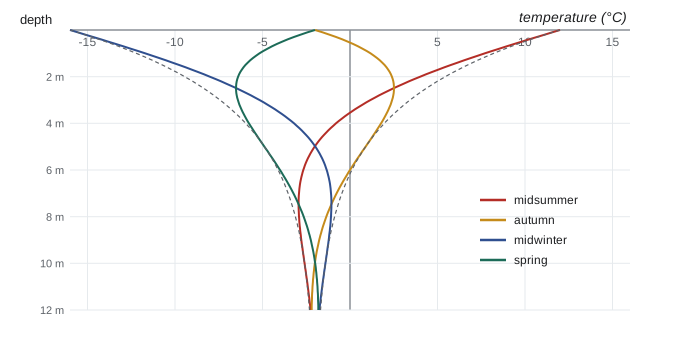
Where is the ground frozen?

The maximum temperature over the year at depth \(z\) is \(T_m + Ae^{-z/d}\). Ground thaws in summer wherever this exceeds 0 °C, which in the purely conductive model happens for

That is far deeper than the active layers observed in such terrain, typically between 0.5 and 2 metres. The model has left out the most important physics of freezing ground: water. A cubic metre of silt holding 30 hundredths of its volume as ice needs about \(0.3 \times 1000 \times 334{,}000 \approx 10^8\) joules to melt, enough to warm the same volume of frozen soil by about 50 °C. Latent heat acts as an enormous thermal buffer at 0 °C, and it is the reason permafrost persists under summers that our linear model says should thaw it deeply.

Stefan's model of the thaw front

Josef Stefan studied the growth of sea ice in 1889, and his model is the classical treatment of a moving phase boundary. Suppose the surface is held at a temperature \(T_s > 0\) during the summer, the ground below the thaw front \(z = X(t)\) is at 0 °C, and heat conducts through the thawed layer with conductivity \(k\). If the thawed layer is thin enough that the temperature in it is nearly linear, the heat flux arriving at the front is \(kT_s/X\). It melts ice at the rate \(L_v\dot X\), where \(L_v\) is the volumetric latent heat. The Stefan condition \(L_v\dot X = kT_s/X\) integrates to

where \(I\) is the thawing index, the accumulated degree-time above freezing, so that a varying surface temperature is allowed. The thaw depth grows like the square root of time, the signature of diffusion. For our surface, the temperature is above 0 °C for the fraction of the year where \(\cos\omega t > 1/7\), and the thawing index is \(\frac1\omega\int_{-\theta}^{\theta}(-2 + 14\cos\phi)\,d\phi\) with \(\theta = \arccos(1/7)\), about 1,280 degree-days. With \(k = 1.2\) W/(m·K) for thawed silt and \(L_v = 10^8\) J/m³,

in line with observations. The Stefan problem is a free boundary problem: the location \(X(t)\) of the boundary is part of the unknown, which makes it nonlinear even though the heat equation on either side is linear. Franz Neumann found an exact similarity solution for a constant surface temperature in the 1860s, and the Stefan formula is its limit when latent heat dominates sensible heat, which is precisely the situation in ice-rich soil.

Geothermal heat and the base of permafrost

Deep down, the Earth's internal heat flows upward at about \(q = 0.06\) W/m². In frozen ground with conductivity \(k_f \approx 2\) W/(m·K), Fourier's law gives a steady gradient \(G = q/k_f = 0.03\) °C/m. Since the heat equation is linear, this steady solution \(Gz\) simply adds to the periodic one:

Below the seasonal layer the temperature rises linearly and reaches 0 °C at \(z_b = |T_m|/G \approx 67\) m, the base of permafrost. Warmer sites, with \(T_m\) closer to zero, have thinner permafrost; at very cold sites in the high Arctic it extends to depths of several hundred metres. The superposition of a steady solution and a periodic one is the method of lesson 7 in a new setting.

A numerical check

The explicit scheme of lesson 11 can solve the full problem with the geothermal flux imposed at the bottom of a finite column and any surface history we like. The program below runs a 30 m column for twelve years from a simple initial state, compares the final years with the exact periodic solution, computes the thawing index and Stefan depth, and finally applies a sudden warming of the mean surface temperature by 1 °C to see how far the signal penetrates.

import math

alpha, year = 1.0e-6, 365.0 * 86400
omega = 2 * math.pi / year
Tm, A, G = -2.0, 14.0, 0.03
d = math.sqrt(2 * alpha / omega)
exact = lambda z, t: Tm + G * z + A * math.exp(-z / d) * math.cos(omega * t - z / d)
print(f"damping depth d = {d:.3f} m, lag at 10 m = {10 / d / omega / 86400:.0f} days, amplitude at 10 m = {A * math.exp(-10 / d):.2f} C")
print(f"depth of 0.1 C amplitude = {d * math.log(A / 0.1):.1f} m, conductive thaw limit = {d * math.log(A / abs(Tm)):.2f} m, permafrost base = {abs(Tm) / G:.0f} m")

# explicit finite differences on 0 <= z <= 30 m, flux u_z = G at the bottom (ghost point)
H, N = 30.0, 120
dz = H / N
dt = 0.25 * 86400
r = alpha * dt / dz ** 2
assert r <= 0.5, r
u = [Tm + G * j * dz for j in range(N + 1)]
steps_per_year = round(year / dt)
t = 0.0
record = {}
for n in range(12 * steps_per_year):
    t += dt
    new = u[:]
    for j in range(1, N):
        new[j] = u[j] + r * (u[j + 1] - 2 * u[j] + u[j - 1])
    new[N] = u[N] + r * (2 * u[N - 1] + 2 * G * dz - 2 * u[N])
    new[0] = Tm + A * math.cos(omega * t)
    u = new
    if n >= 11 * steps_per_year:                  # last year: record extremes
        for zz in (1, 2, 5, 10):
            j = round(zz / dz)
            lo, hi = record.get(zz, (99, -99))
            record[zz] = (min(lo, u[j]), max(hi, u[j]))
print(f"r = {r:.3f}")
for zz, (lo, hi) in record.items():
    print(f"z = {zz:2d} m: model range {lo:+.2f} to {hi:+.2f} C, exact {Tm + G * zz - A * math.exp(-zz / d):+.2f} to {Tm + G * zz + A * math.exp(-zz / d):+.2f} C")
err = max(abs(u[j] - exact(j * dz, t)) for j in range(N + 1))
print(f"max difference from exact periodic solution at the end: {err:.3f} C")

# thawing index and Stefan thaw depth
theta = math.acos(abs(Tm) / A)
I = (-2 * abs(Tm) * theta + 2 * A * math.sin(theta)) / omega        # degree-seconds
k, Lv = 1.2, 0.30 * 1000 * 334000
print(f"thawing index {I / 86400:.0f} degree-days, thaw season {2 * theta / omega / 86400:.0f} days, Stefan depth {math.sqrt(2 * k * I / Lv):.2f} m")

# a step warming of 1 C at the surface: excess temperature erfc(z / (2 sqrt(alpha t)))
for yrs in (10, 30, 100):
    tt = yrs * year
    row = "  ".join(f"{z} m: {math.erfc(z / (2 * math.sqrt(alpha * tt))):.2f}" for z in (10, 25, 50, 100))
    print(f"after {yrs:3d} years of warming, fraction felt at  {row}")

damping depth d = 3.168 m, lag at 10 m = 183 days, amplitude at 10 m = 0.60 C
depth of 0.1 C amplitude = 15.7 m, conductive thaw limit = 6.17 m, permafrost base = 67 m
r = 0.346
z =  1 m: model range -12.18 to +8.24 C, exact -12.18 to +8.24 C
z =  2 m: model range -9.39 to +5.51 C, exact -9.39 to +5.51 C
z =  5 m: model range -4.74 to +1.04 C, exact -4.74 to +1.04 C
z = 10 m: model range -2.30 to -1.10 C, exact -2.30 to -1.10 C
max difference from exact periodic solution at the end: 0.003 C
thawing index 1278 degree-days, thaw season 166 days, Stefan depth 1.63 m
after  10 years of warming, fraction felt at  10 m: 0.69  25 m: 0.32  50 m: 0.05  100 m: 0.00
after  30 years of warming, fraction felt at  10 m: 0.82  25 m: 0.57  50 m: 0.25  100 m: 0.02
after 100 years of warming, fraction felt at  10 m: 0.90  25 m: 0.75  50 m: 0.53  100 m: 0.21

After a dozen years the numerical model has forgotten its initial state and matches the exact periodic solution to within a few thousandths of a degree, with the seasonal ranges at each depth in agreement. The Stefan estimate of about 1.6 m for the thaw depth is far shallower than the 6.2 m of the purely conductive model, the effect of latent heat. The last table uses the half-space solution \(\Delta T\,\mathrm{erfc}\big(z/(2\sqrt{\alpha t})\big)\) for a sudden surface warming \(\Delta T\), found by the similarity variable \(z/\sqrt{t}\) or by the Fourier transform: after 30 years, half of the warming is felt at about 30 m, and after a century half of it is felt at more than 50 m.

Reading the climate from boreholes

The slow downward diffusion of surface warming has a remarkable consequence. A temperature profile measured in a borehole today is a record of past surface temperatures, smeared by diffusion, much as a footprint in sand records a step. In 1986 Arthur Lachenbruch and Vaughn Marshall showed that temperature profiles in oil-exploration boreholes in northern Alaska curved away from the steady geothermal line in the upper hundred metres, and inverted them to infer a surface warming of several degrees over the preceding century. Reconstructing a past surface history from a present profile is a backward heat problem, ill posed in exactly the sense of Hadamard (lesson 1): only smooth, long-term features of the past can be recovered, and regularization methods are needed to stop high-frequency noise from swamping the answer.

What the model teaches

Each stage of the model used a different tool from the course. The heat equation came from conservation of energy and Fourier's law (lesson 4). The periodic solution used separation of variables in complex form, and its exponential decay with depth mirrors the hyperbolic decay into the interior of a plate in lesson 9. The damping depth is a diffusion length \(\sqrt{\alpha\tau}\), the square-root scaling of lesson 4 again. Superposing the geothermal gradient used linearity, as in lesson 7. The numerical check needed the stability condition \(r \le \frac12\) of lesson 11. The step-warming solution is the half-space version of the heat kernel. And the limitations, latent heat and the moving thaw front, point beyond linear PDEs to free boundary problems, where much current research lies. Engineers working in the North use exactly these ideas, in more elaborate numerical form, to decide how deep to set piles, how thick to make gravel pads under roads, and when thermosyphons are needed to keep the ground under a building frozen.