First-order PDEs and the method of characteristics

First-order equations are the natural place to begin solving PDEs, because they can be reduced exactly to ordinary differential equations. The idea is geometric. A first-order linear equation such as \(a\,u_x + b\,u_y = 0\) says that the directional derivative of \(u\) in the direction \((a, b)\) is zero, so \(u\) is constant along lines in that direction. Those lines are the characteristics of the equation, and along them the PDE becomes an ODE. This lesson develops the method of characteristics for linear, variable-coefficient and quasilinear equations, uses it to model traffic and pollutant transport, and shows how nonlinear equations can form shocks in finite time.

The transport equation

The simplest first-order PDE is the transport or advection equation

with constant speed \(c\). It models a substance carried along by a fluid moving at velocity \(c\), such as a dissolved pollutant in a river, if diffusion is neglected. Consider the lines \(x = x_0 + ct\) in the \((x, t)\) plane. Along such a line, by the chain rule,

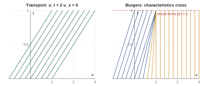
so \(u\) is constant along the line and equals its starting value \(f(x_0)\). Since \(x_0 = x - ct\), the solution is \(u(x, t) = f(x - ct)\): the initial profile translates to the right at speed \(c\) without changing shape. Every point of the \((x, t)\) plane lies on exactly one characteristic line, which traces back to a unique point of the initial line, so the solution exists and is unique for every differentiable \(f\). When \(f\) has a corner or a jump, the formula still makes sense and describes a corner or jump travelling along a characteristic. Such functions are not classical solutions, but they are weak solutions in a sense made precise later in the subject, and physically they are exactly right.

General linear first-order equations

Now consider the linear equation with variable coefficients

The left side's first two terms form the derivative of \(u\) along curves whose tangent is \((a, b)\). Parametrize such a curve by \(s\) and solve the characteristic system

The first two equations determine the characteristic curves in the \((x, y)\) plane independently of \(u\). The third is a linear ODE for \(u\) along each curve. The data are given on an initial curve \(\Gamma\), and each characteristic starts on \(\Gamma\) with the prescribed value of \(u\). For the construction to work, the characteristics must cross \(\Gamma\) rather than run along it. If \(\Gamma\) is itself a characteristic at some point, the data there cannot be chosen freely, because the PDE already dictates how \(u\) changes along \(\Gamma\); we say \(\Gamma\) is characteristic, and the problem typically has no solution or infinitely many.

An equivalent formulation eliminates the parameter: the characteristic curves satisfy \(dy/dx = b/a\). For the homogeneous equation with \(c = g = 0\), every first integral \(\xi(x, y) = \text{constant}\) of this ODE gives a family of characteristics, and the general solution is \(u = F(\xi(x, y))\) for an arbitrary function \(F\). As in lesson 1, arbitrary functions replace arbitrary constants.

Quasilinear equations and traffic flow

A first-order equation is quasilinear if it is linear in the derivatives but the coefficients may depend on \(u\):

The characteristic system \(dx/ds = a\), \(dy/ds = b\), \(du/ds = g\) is now coupled: the curves depend on the solution. The most important example is a conservation law. Let \(\rho(x, t)\) be the density of cars on a highway, in cars per kilometre, and \(q(\rho)\) the flux, in cars per hour passing a point. Conservation of cars between two points \(a < b\) says \(\frac{d}{dt}\int_a^b \rho\,dx = q(a) - q(b)\), and letting \(b \to a\) gives \(\rho_t + q(\rho)_x = 0\), or

In the model of Lighthill, Whitham and Richards (1955–56) the speed of cars decreases linearly with density, \(v = v_{\max}(1 - \rho/\rho_{\max})\), so \(q = \rho v\) is a downward parabola and the characteristic speed \(q'(\rho) = v_{\max}(1 - 2\rho/\rho_{\max})\) is positive in light traffic and negative in heavy traffic. That is why a disturbance in dense traffic, such as brake lights, travels backward along the highway even though every car is moving forward. Along each characteristic \(\rho\) is constant, so the characteristics are straight lines, but their slopes depend on the initial density where they start.

The inviscid Burgers equation and shocks

The simplest nonlinear conservation law is the inviscid Burgers equation, named for Johannes Burgers, who used it in the 1940s as a model of turbulence:

The characteristic speed is \(u\) itself. Along \(x = x_0 + f(x_0)\,t\), the value of \(u\) is constant and equal to \(f(x_0)\), so the solution is given implicitly by \(u = f(x - ut)\). Where \(f\) is increasing, faster characteristics start ahead of slower ones and spread out, forming a rarefaction. Where \(f\) is decreasing, faster characteristics start behind slower ones and eventually catch them. When two characteristics cross, they carry different values of \(u\) to the same point, and the classical solution breaks down. Differentiating the implicit solution gives

which blows up when \(t = -1/f'(x_0)\). The first breaking time is therefore \(t_b = -1/\min f'\), defined when \(f\) decreases somewhere. Beyond \(t_b\) the physically relevant solution contains a jump called a shock. Its speed is determined by conservation of \(u\) across it; for the Burgers equation, with flux \(u^2/2\), the Rankine–Hugoniot condition gives the shock speed \(s = (u_L + u_R)/2\), the average of the states on either side.

Computing along characteristics

When the characteristic ODEs cannot be solved by hand, they can be integrated numerically: start from many points on the initial curve, march each characteristic forward with a standard ODE solver, and read off \(u\) at the end. The program below does this for the rotating flow and for the variable-speed equation \(u_t + x\,u_x = 0\), whose characteristics \(x = x_0e^t\) fan out exponentially, and compares with exact solutions. It then solves the Burgers equation implicitly by fixed-point iteration on \(u = f(x - ut)\) before the breaking time.

import math

def rk4(F, y, s, h):
    k1 = F(s, y)
    k2 = F(s + h/2, [a + h/2*b for a, b in zip(y, k1)])
    k3 = F(s + h/2, [a + h/2*b for a, b in zip(y, k2)])
    k4 = F(s + h, [a + h*b for a, b in zip(y, k3)])
    return [a + h/6*(p + 2*q + 2*r + w) for a, p, q, r, w in zip(y, k1, k2, k3, k4)]

def follow(F, y0, S, n=400):
    y, h = list(y0), S / n
    for i in range(n):
        y = rk4(F, y, i*h, h)
    return y

# 1) -y u_x + x u_y = 0 with u(x,0) = exp(-x^2): march (x, y, u) around the circle
F = lambda s, y: [-y[1], y[0], 0.0]
for x0 in (0.5, 1.0, 1.5):
    x, y, u = follow(F, [x0, 0.0, math.exp(-x0**2)], math.pi/3)
    print(f"rotation: start x0={x0}, end ({x:+.4f},{y:+.4f}), u={u:.5f}, exact {math.exp(-(x*x+y*y)):.5f}")

# 2) u_t + x u_x = 0, u(x,0) = 1/(1+x^2): exact u = 1/(1 + x^2 e^{-2t})
F2 = lambda s, y: [y[0], 1.0, 0.0]          # dx/ds = x, dt/ds = 1, du/ds = 0
for x0 in (0.2, 0.6, 1.0):
    x, t, u = follow(F2, [x0, 0.0, 1/(1 + x0**2)], 1.0)
    print(f"stretching: x0={x0} -> x={x:.5f} at t=1, u={u:.5f}, exact {1/(1 + x*x*math.exp(-2)):.5f}")

# 3) Burgers u_t + u u_x = 0 with a smooth decreasing profile; solve u = f(x - u t)
f = lambda x: 0.5 * (1 - math.tanh(x))
fp_min = min((f(z + 1e-6) - f(z - 1e-6)) / 2e-6 for z in [k/100 for k in range(-300, 301)])
print(f"breaking time t_b = -1/min f' = {-1/fp_min:.4f} (exact 2)")
def burgers(x, t):
    u = f(x)
    for _ in range(200):
        u = 0.5*u + 0.5*f(x - u*t)          # damped fixed-point iteration
    return u
for t in (0.0, 1.0, 1.8):
    vals = [burgers(-1 + 0.5*k, t) for k in range(6)]
    print(f"t={t}: " + "  ".join(f"{v:.3f}" for v in vals))

rotation: start x0=0.5, end (+0.2500,+0.4330), u=0.77880, exact 0.77880
rotation: start x0=1.0, end (+0.5000,+0.8660), u=0.36788, exact 0.36788
rotation: start x0=1.5, end (+0.7500,+1.2990), u=0.10540, exact 0.10540
stretching: x0=0.2 -> x=0.54366 at t=1, u=0.96154, exact 0.96154
stretching: x0=0.6 -> x=1.63097 at t=1, u=0.73529, exact 0.73529
stretching: x0=1.0 -> x=2.71828 at t=1, u=0.50000, exact 0.50000
breaking time t_b = -1/min f' = 2.0000 (exact 2)
t=0.0: 0.881  0.731  0.500  0.269  0.119  0.047
t=1.0: 0.981  0.948  0.844  0.500  0.156  0.052
t=1.8: 0.996  0.990  0.971  0.905  0.249  0.058

The numerical characteristics reproduce the exact solutions to five decimal places. For the smooth profile \(f(x) = (1 - \tanh x)/2\), the steepest slope is \(-1/2\) at \(x = 0\), giving breaking time 2; the table shows the profile steepening as \(t\) approaches it. Beyond that time the fixed-point iteration would have several solutions to choose from, which is the analytic signature of crossing characteristics.

The general first-order equation

Fully nonlinear first-order equations \(F(x, y, u, u_x, u_y) = 0\), such as the eikonal equation \(u_x^2 + u_y^2 = 1\) of geometric optics, can also be solved by characteristics, but now the system must carry the derivatives \(p = u_x\) and \(q = u_y\) along as well. The resulting Charpit–Lagrange equations,

describe rays in optics and the paths of least time. Hamilton's development of these equations in the 1820s and 1830s connected wave fronts and particle mechanics and later shaped quantum mechanics. For the eikonal equation the rays are straight lines perpendicular to the wave fronts, and \(u\) measures distance travelled. We will not need the general theory again, but it shows how far the characteristic idea reaches.

Characteristics will return in lesson 3, where the second-order equations are classified by how many real characteristic directions they have, and in lesson 8, where the wave equation factors into two transport equations whose characteristics are the lines \(x \pm ct = \text{constant}\). The numerical schemes of lesson 11 must also respect characteristics: an explicit scheme that ignores the direction in which information travels cannot be stable.