What partial differential equations describe

An ordinary differential equation describes a quantity that depends on one variable, usually time: the charge on a capacitor, the population of a species, the angle of a pendulum. Most of the physical world is not like that. The temperature in a room depends on where you stand as well as when you look; the height of a guitar string depends on the position along the string and on time; the electric potential around a charged conductor depends on three coordinates in space. A law that links the rates of change of such a quantity in several directions at once is a partial differential equation, or PDE. This course is about the three classical PDEs of mathematical physics, the heat, wave and Laplace equations, and the methods that solve them: characteristics, Fourier series, separation of variables, special functions and finite differences. This first lesson fixes the vocabulary, shows what the three model equations do, and explains why a PDE alone is never a complete problem.

Notation and vocabulary

A partial differential equation for an unknown function \(u(x, t)\) or \(u(x, y)\) is a relation between \(u\), its independent variables and finitely many of its partial derivatives. We write subscripts for partial derivatives: \(u_t = \partial u/\partial t\), \(u_x = \partial u/\partial x\), \(u_{xx} = \partial^2 u/\partial x^2\) and \(u_{xy} = \partial^2 u/\partial x\,\partial y\). For a function of several space variables the Laplacian is the sum of the unmixed second derivatives, \(\Delta u = u_{xx} + u_{yy}\) in the plane and \(\Delta u = u_{xx} + u_{yy} + u_{zz}\) in space. The gradient \(\nabla u\) is the vector of first partial derivatives, and the divergence of a vector field \(\mathbf F = (F_1, F_2, F_3)\) is \(\nabla \cdot \mathbf F = \partial_x F_1 + \partial_y F_2 + \partial_z F_3\), so that \(\Delta u = \nabla \cdot \nabla u\).

The order of a PDE is the order of the highest derivative that appears. The transport equation \(u_t + c\,u_x = 0\) is first order; the heat equation \(u_t = \alpha u_{xx}\) is second order, even though it contains only a first derivative in time; the beam equation \(u_{tt} + EI\,u_{xxxx} = 0\) is fourth order. An equation is linear if it has the form \(\mathcal L u = f\), where \(\mathcal L\) is a linear differential operator, meaning \(\mathcal L(au + bv) = a\mathcal L u + b\mathcal L v\) for all functions \(u\), \(v\) and constants \(a\), \(b\). The coefficients of a linear operator may depend on the independent variables but not on \(u\). A linear equation is homogeneous when \(f = 0\) and inhomogeneous otherwise. Equations that are linear in the highest derivatives but not otherwise are called semilinear or quasilinear; the Burgers equation \(u_t + u\,u_x = 0\), which lesson 2 studies, is quasilinear, and the minimal surface equation is fully nonlinear in spirit.

Linearity is the single most useful property a PDE can have, because of the superposition principle: if \(u_1, \ldots, u_N\) solve the homogeneous equation \(\mathcal L u = 0\), so does every linear combination \(c_1u_1 + \cdots + c_Nu_N\). Fourier series, the heart of this course, extend superposition to infinite sums. A second consequence is that the general solution of an inhomogeneous linear problem is one particular solution plus the general solution of the homogeneous problem, exactly as for linear ODEs.

The three model equations

Three second-order linear equations dominate the subject. Each is the prototype of a whole class, and lesson 3 shows that every second-order linear equation in two variables behaves locally like one of them.

The heat equation, also called the diffusion equation, governs the temperature in a conducting solid, the concentration of a dye spreading in still water, and the probability density of a particle undergoing Brownian motion. The constant \(\alpha > 0\) is the diffusivity, with units of area per time. Its defining feature is smoothing: sharp corners in the initial temperature are rounded off instantly, and differences in temperature decay as time goes on. The equation is not reversible in time; running it backwards amplifies small wiggles without bound, which is the mathematical face of the second law of thermodynamics.

The wave equation governs small vibrations of a string or membrane, sound in air, and electromagnetic fields in empty space. The constant \(c\) is the wave speed. Where the heat equation smooths, the wave equation transports: a disturbance travels at speed \(c\) and keeps its shape, corners included. The equation is reversible, since replacing \(t\) by \(-t\) leaves it unchanged, and it conserves an energy, a fact lesson 8 proves.

Laplace's equation describes equilibrium. If the temperature in a body has stopped changing, \(u_t = 0\) and the heat equation reduces to \(\Delta u = 0\). The same equation governs electrostatic potential in a region free of charge, the velocity potential of an ideal fluid, and the steady seepage of groundwater. Its solutions, the harmonic functions, are as smooth as functions can be, and they obey a maximum principle: a harmonic function on a bounded region takes its largest and smallest values on the boundary. Adding a source term gives Poisson's equation \(\Delta u = f\), named for Siméon Denis Poisson, who studied it in 1813 in connection with gravitational potential inside matter.

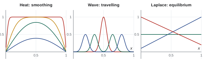
In one space dimension Laplace's equation is simply \(u'' = 0\), whose solutions are straight lines. A rod whose ends are held at temperatures \(a\) and \(b\) eventually settles to the linear profile \(u = a + (b - a)x/L\), whatever its initial state. The interesting behaviour of harmonic functions, such as the mean value property and the smoothing of boundary data into the interior, only appears in two or more dimensions.

Checking that a function is a solution

A classical solution of a second-order PDE on an open region is a function that has continuous derivatives up to second order there and satisfies the equation at every point. Checking a candidate is a matter of differentiation, and doing so a few times builds intuition about what each equation allows.

Observe how much freedom the wave equation allows: an arbitrary function \(F\) produces a solution. The general solution of a PDE typically involves arbitrary functions rather than arbitrary constants, which is one reason PDEs are harder than ODEs. To pin down a single solution we need much more information than a few numbers.

Initial and boundary conditions

A PDE becomes a solvable problem only when it is supplemented with side conditions that describe the particular physical situation. For an evolution equation in time we prescribe an initial condition. The heat equation is first order in time and needs one, the initial temperature \(u(x, 0) = f(x)\). The wave equation is second order in time and needs two, the initial displacement \(u(x, 0) = f(x)\) and the initial velocity \(u_t(x, 0) = g(x)\), just as Newton's second law needs an initial position and velocity.

On a bounded region we also need boundary conditions on the edge, for all times. For a rod occupying \(0 \le x \le L\), the three standard types are:

Dirichlet conditions prescribe the value of \(u\) on the boundary, such as \(u(0, t) = T_0\) for an end held in ice water. They are named for Peter Gustav Lejeune Dirichlet. Neumann conditions, named for Carl Neumann, prescribe the normal derivative, such as \(u_x(L, t) = 0\) for an insulated end through which no heat flows. Robin conditions prescribe a combination, \(u_x + h u = 0\), which models an end that loses heat to its surroundings at a rate proportional to its temperature, as in Newton's law of cooling. For Laplace's equation on a region there is no initial condition; the boundary data alone determine the solution. The pairing of an equation with conditions gives names such as initial value problem, boundary value problem and initial-boundary value problem.

Well-posed problems

In 1902 Jacques Hadamard proposed that a mathematical model of a physical process should be well posed: a solution should exist, it should be unique, and it should depend continuously on the data, so that small errors in measurement produce small errors in the prediction. The third requirement is subtle but essential, because data are never known exactly. The heat equation run forward in time with a temperature given at \(t = 0\) is well posed. Run backward, it is not.

Hadamard's own example shows that the wrong side conditions can destroy well-posedness even for Laplace's equation. Consider \(u_{xx} + u_{yy} = 0\) for \(y > 0\), treated as an evolution in \(y\), with data \(u(x, 0) = 0\) and \(u_y(x, 0) = \sin(nx)/n\). The solution is \(u = \sinh(ny)\sin(nx)/n^2\). As \(n \to \infty\) the data tend uniformly to zero, but for any fixed \(y > 0\) the solution grows like \(e^{ny}/n^2\), which is unbounded. Tiny changes in the data produce enormous changes in the solution, so this Cauchy problem for Laplace's equation is ill posed. Equilibrium problems want boundary data all the way round, not initial data on one side.

A common way to prove uniqueness is the energy method. Suppose \(u_1\) and \(u_2\) both solve the heat equation on \(0 < x < L\) with the same initial and Dirichlet boundary data. Their difference \(w\) solves the heat equation with zero data. Let \(E(t) = \int_0^L w^2\,dx\). Then

because the boundary term vanishes. So \(E\) is non-increasing, \(E(0) = 0\) and \(E \ge 0\), which forces \(E(t) = 0\) for all \(t\) and \(w \equiv 0\). The same calculation with nonzero data gives a bound on how fast two solutions can separate, which is continuous dependence measured in the mean-square sense.

A short history

Partial differential equations entered mathematics in the eighteenth century through vibrating strings. Jean le Rond d'Alembert derived the one-dimensional wave equation and its general solution as a sum of left- and right-moving waves in 1747. Leonhard Euler promptly extended the solution to initial shapes with corners, which d'Alembert refused to accept, and Daniel Bernoulli argued that every vibration was a superposition of sinusoidal modes. The resulting controversy, about what counts as a function, was not settled for a century. Pierre-Simon Laplace used the equation that bears his name in his work on celestial mechanics and gravitational potential from the 1780s onward, although Euler had written it earlier in hydrodynamics.

Joseph Fourier presented his theory of heat conduction to the Paris Academy in 1807, derived the heat equation from a law of heat flux, and claimed that any initial temperature could be represented by a trigonometric series. The memoir met resistance from Lagrange and Laplace, won a prize in 1812, and was finally published as the book Théorie analytique de la chaleur in 1822. Making Fourier's claim precise drove much of nineteenth-century analysis: Dirichlet's convergence theorem of 1829, Riemann's integral, Cantor's set theory and eventually Lebesgue's integral all grew from questions about Fourier series. In the twentieth century computers made numerical methods central. The 1928 paper of Richard Courant, Kurt Friedrichs and Hans Lewy on difference equations, and the 1947 scheme of John Crank and Phyllis Nicolson for the heat equation, are the foundations of lesson 11.

Computing with a PDE solution

Throughout the course we check analytic results with short Python programs that use only the standard library. The first program verifies the three families from the worked example numerically: it approximates the derivatives by centred differences at a sample point and reports the residual of each equation, which should be close to zero up to rounding and truncation error.

import math

def d1(f, x, h=1e-4):
    return (f(x + h) - f(x - h)) / (2 * h)
def d2(f, x, h=1e-3):
    return (f(x + h) - 2 * f(x) + f(x - h)) / (h * h)

alpha, k, c = 0.7, 3.0, 2.0
heat = lambda x, t: math.exp(-alpha * k * k * t) * math.sin(k * x)
F = lambda z: math.exp(-z * z)               # any smooth profile
wave = lambda x, t: F(x - c * t)
lap = lambda x, y: math.log(x * x + y * y)

x0, t0, y0 = 0.4, 0.3, 0.9
r_heat = d1(lambda t: heat(x0, t), t0) - alpha * d2(lambda x: heat(x, t0), x0)
r_wave = d2(lambda t: wave(x0, t), t0) - c * c * d2(lambda x: wave(x, t0), x0)
r_lap = d2(lambda x: lap(x, y0), x0) + d2(lambda y: lap(x0, y), y0)
print(f"heat residual    {r_heat:+.2e}")
print(f"wave residual    {r_wave:+.2e}")
print(f"Laplace residual {r_lap:+.2e}")

# a function that is NOT harmonic, for contrast
bad = lambda x, y: x * x + y * y
print(f"x^2 + y^2 gives  {d2(lambda x: bad(x, y0), x0) + d2(lambda y: bad(x0, y), y0):+.4f}  (Laplacian = 4)")

# decay rates: higher wavenumbers die faster under heat flow
for kk in (1, 2, 4, 8):
    print(f"k = {kk}: amplitude after t = 0.1 is {math.exp(-alpha * kk * kk * 0.1):.4f}")

heat residual    -7.24e-07
wave residual    +9.71e-06
Laplace residual +2.17e-07
x^2 + y^2 gives  +4.0000  (Laplacian = 4)
k = 1: amplitude after t = 0.1 is 0.9324
k = 2: amplitude after t = 0.1 is 0.7558
k = 4: amplitude after t = 0.1 is 0.3263
k = 8: amplitude after t = 0.1 is 0.0113

The residuals are of the order of the difference approximations' truncation error, about \(10^{-6}\), while the non-harmonic function \(x^2 + y^2\) gives a Laplacian of 4. The decay table previews the central fact about heat flow: a component with wavenumber 8 decays by a factor of nearly 90 in the time it takes the wavenumber 1 component to lose 7 parts in 100 of its size. Lesson 11 turns the difference approximations used here into complete numerical solvers.

Where PDEs come from

Most PDEs of physics arise by combining a conservation law with a constitutive law. The conservation law says that the rate of change of the amount of something in a region equals the net flow across its boundary plus whatever is produced inside. It is exact and universal. The constitutive law relates the flow to the state, for example Fourier's law that heat flows from hot to cold at a rate proportional to the temperature gradient, or Fick's law for diffusing chemicals, or Darcy's law for groundwater. It is empirical and specific to a material. Lesson 4 carries out this derivation for heat and for a vibrating string. The same pattern produces the equations of fluid dynamics, elasticity, traffic flow, population dispersal and option pricing: the Black–Scholes equation of finance is a heat equation in disguise.

Because the same few equations recur in so many fields, the methods of this course transfer directly. A Fourier series that solves a heat problem also solves a diffusion problem in chemistry; a Bessel function that describes a vibrating drum also describes heat flow in a cylinder and electromagnetic modes in a circular waveguide. Learning the methods once pays off many times over.