Classifying second-order PDEs: elliptic, parabolic and hyperbolic

The heat, wave and Laplace equations look alike on paper, each a short combination of second derivatives, yet lesson 1 showed that they behave in completely different ways. This lesson explains why. Every second-order linear equation in two variables can be sorted by the sign of a single number, its discriminant, into one of three types named after the conic sections: elliptic, like Laplace's equation; parabolic, like the heat equation; and hyperbolic, like the wave equation. The type decides which side conditions make a well-posed problem, how fast information travels and how smooth solutions are. A change of variables brings each type to a standard canonical form, and the construction of those variables is another application of characteristics.

The general second-order linear equation

Consider the equation

where the coefficients may depend on \(x\) and \(y\). The second-order terms, called the principal part, determine the type. By analogy with the conic \(Ax^2 + Bxy + Cy^2 = 1\), define the discriminant \(\Delta = B^2 - 4AC\). At a point where

Laplace's equation \(u_{xx} + u_{yy} = 0\) has \(A = C = 1\), \(B = 0\) and discriminant \(-4\): elliptic. The heat equation written as \(\alpha u_{xx} - u_t = 0\), with \(y = t\), has \(A = \alpha\), \(B = C = 0\) and discriminant 0: parabolic. The wave equation \(u_{tt} - c^2u_{xx} = 0\) has \(A = -c^2\), \(B = 0\), \(C = 1\) and discriminant \(4c^2 > 0\): hyperbolic. The lower-order terms play no role in the classification, though they matter a great deal for the solutions. With variable coefficients the type can change from point to point.

Some authors use the convention \(A\,u_{xx} + 2B\,u_{xy} + C\,u_{yy}\), in which case the discriminant becomes \(B^2 - AC\). The two conventions agree in sign, so the classification is the same. Here we keep the coefficient \(B\) of \(u_{xy}\) as it stands.

Characteristics of a second-order equation

The classification has a geometric meaning. Suppose we try to solve the equation near a curve \(\Gamma\) on which \(u\) and its normal derivative are prescribed, the Cauchy problem. Knowing \(u\) and \(u_n\) along \(\Gamma\) gives \(u_x\) and \(u_y\) there, and differentiating along \(\Gamma\) gives two linear equations for the three second derivatives. The PDE supplies a third. If the three equations can be solved, we know all second derivatives on \(\Gamma\), and the process continues to higher orders, determining a power series solution. The system fails to be solvable exactly when the direction \((dx, dy)\) of \(\Gamma\) satisfies

Curves whose tangent satisfies this condition are the characteristic curves of the equation. Dividing by \((dx)^2\) gives a quadratic for the slope, \(A\,(dy/dx)^2 - B\,(dy/dx) + C = 0\), with roots

A hyperbolic equation has two distinct real families of characteristics, a parabolic equation has one, and an elliptic equation has none. For the wave equation \(u_{tt} = c^2u_{xx}\) the characteristics are the lines \(x \pm ct = \text{constant}\), along which signals travel. For the heat equation the only characteristics are the lines \(t = \text{constant}\), which is why initial data are given on such a line and why heat appears to propagate infinitely fast. For Laplace's equation there are no real characteristics, so no curve can carry independent data, and Cauchy data on an open curve lead to Hadamard's ill-posed problem.

Canonical forms

A smooth change of variables \(\xi = \xi(x, y)\), \(\eta = \eta(x, y)\) with nonzero Jacobian turns the equation into one of the same form in the new variables, with new coefficients \(A^*\), \(B^*\), \(C^*\). A direct computation with the chain rule shows

so the sign of the discriminant, and hence the type, does not depend on the coordinates. The idea is to choose \(\xi\) and \(\eta\) so as to kill as many second-order coefficients as possible. If \(\xi\) is constant along one family of characteristics, then \(A^* = 0\), because the condition \(A\xi_x^2 + B\xi_x\xi_y + C\xi_y^2 = 0\) is exactly the characteristic equation for the level curves of \(\xi\). This gives the three canonical forms, where dots stand for terms of lower order:

For a hyperbolic equation, take \(\xi\) and \(\eta\) constant along the two characteristic families; then \(A^* = C^* = 0\). For a parabolic equation there is only one family, so take \(\xi\) constant along it and \(\eta\) any independent function; then \(A^* = 0\), and \(B^* = 0\) follows automatically from the zero discriminant. For an elliptic equation with analytic coefficients, the characteristic roots are complex conjugates, and taking the real and imaginary parts of a complex characteristic variable gives the Laplacian form.

Equations that change type

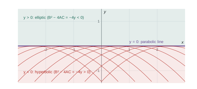
With variable coefficients the discriminant can change sign. The Tricomi equation \(y\,u_{xx} + u_{yy} = 0\), studied by Francesco Tricomi in 1923, has \(A = y\), \(B = 0\), \(C = 1\), so \(B^2 - 4AC = -4y\). It is elliptic in the upper half-plane, hyperbolic in the lower half-plane and parabolic on the \(x\)-axis. Its characteristics in the hyperbolic region satisfy \((dy/dx)^2 = -1/y\), which integrates to the cusped curves \(\frac{3}{2}(x - x_0) = \pm(-y)^{3/2}\) meeting the axis at right angles. The equation arises in transonic gas dynamics: the flow over an aircraft wing near the speed of sound is subsonic (elliptic) in some regions and supersonic (hyperbolic) in others, and the change of type is where shock waves appear. The closely related equation \(u_{xx} + y\,u_{yy} = 0\) has the same discriminant \(-4y\) and the same pattern of types; its characteristics satisfy \((dy/dx)^2 = -y\) and are the parabolas \(y = -(x - c)^2/4\), each touching the axis at \(x = c\), as the figure shows.

What the type tells us

The classification is a guide to what kind of problem makes sense. Hyperbolic equations describe propagation at finite speed. They need Cauchy data, values and normal derivatives, on a non-characteristic curve such as \(t = 0\), and the solution at a point depends only on data in a bounded domain of dependence cut out by the characteristics. Singularities, such as corners and jumps, are carried along characteristics and do not smooth out. Parabolic equations describe diffusion. They need one initial condition and boundary conditions, they smooth their data instantly, and a disturbance is felt everywhere immediately, though only very weakly far away. Elliptic equations describe equilibria. They need boundary data on a closed curve, their solutions are smooth in the interior (analytic, when the coefficients are), and a change of data anywhere on the boundary affects the solution everywhere inside.

The type also shapes numerical methods. For hyperbolic equations, explicit time-stepping works if the time step respects the speed of propagation, the Courant–Friedrichs–Lewy condition of lesson 11. For parabolic equations, explicit stepping requires very small time steps and implicit schemes are usually preferred. Elliptic problems have no time at all; their discretizations are large systems of linear equations solved by iteration, as in lesson 9.

Classifying by computer

For variable coefficients it is useful to scan a region and map the type. The program below classifies the Tricomi equation and a second example, \(u_{xx} + 2x\,u_{xy} + (1 - y^2)u_{yy} = 0\), on a grid, and it checks the invariance of the discriminant's sign under a randomly chosen linear change of variables.

import random

def kind(A, B, C, tol=1e-12):
    d = B*B - 4*A*C
    return 'H' if d > tol else ('E' if d < -tol else 'P')

def show(coef, label):
    print(label)
    for j in range(4, -5, -2):
        y = j / 2
        row = ''.join(kind(*coef(i / 2, y)) for i in range(-6, 7))
        print(f"  y = {y:+.1f}  {row}")

show(lambda x, y: (y, 0.0, 1.0), "Tricomi y u_xx + u_yy  (x from -3 to 3)")
show(lambda x, y: (1.0, 2*x, 1 - y*y), "u_xx + 2x u_xy + (1 - y^2) u_yy")

# invariance: new coefficients under xi = a x + b y, eta = c x + d y
rng = random.Random(336)
for trial in range(3):
    A, B, C = (rng.uniform(-2, 2) for _ in range(3))
    a, b, c, d = (rng.uniform(-2, 2) for _ in range(4))
    As = A*a*a + B*a*b + C*b*b
    Cs = A*c*c + B*c*d + C*d*d
    Bs = 2*A*a*c + B*(a*d + b*c) + 2*C*b*d
    J = a*d - b*c
    lhs, rhs = Bs*Bs - 4*As*Cs, J*J*(B*B - 4*A*C)
    print(f"disc before {B*B-4*A*C:+.4f} ({kind(A,B,C)}), after {lhs:+.4f} ({kind(As,Bs,Cs)}), J^2 * before = {rhs:+.4f}")

Tricomi y u_xx + u_yy  (x from -3 to 3)
  y = +2.0  EEEEEEEEEEEEE
  y = +1.0  EEEEEEEEEEEEE
  y = +0.0  PPPPPPPPPPPPP
  y = -1.0  HHHHHHHHHHHHH
  y = -2.0  HHHHHHHHHHHHH
u_xx + 2x u_xy + (1 - y^2) u_yy
  y = +2.0  HHHHHHHHHHHHH
  y = +1.0  HHHHHHPHHHHHH
  y = +0.0  HHHHPEEEPHHHH
  y = -1.0  HHHHHHPHHHHHH
  y = -2.0  HHHHHHHHHHHHH
disc before +14.1092 (H), after +15.7122 (H), J^2 * before = +15.7122
disc before +0.9222 (H), after +3.3138 (H), J^2 * before = +3.3138
disc before -5.4731 (E), after -1.7708 (E), J^2 * before = -1.7708

For the second equation the discriminant is \(4x^2 - 4(1 - y^2) = 4(x^2 + y^2 - 1)\), so it is elliptic inside the unit circle, parabolic on it and hyperbolic outside: the grid marks P at the four grid points that lie exactly on the circle. The invariance check confirms that the discriminant is multiplied by the squared Jacobian, so its sign never changes.

Higher dimensions and systems

In \(n\) variables the principal part is \(\sum a_{ij}u_{x_ix_j}\) with a symmetric coefficient matrix \(A = (a_{ij})\). The equation is elliptic when all eigenvalues of \(A\) have the same sign, hyperbolic when one eigenvalue has the opposite sign to the other \(n - 1\) (as for \(u_{tt} - c^2\Delta u\)), and parabolic when one eigenvalue is zero and the rest share a sign (as for \(u_t - \alpha\Delta u\)). There are further types in four or more dimensions, called ultrahyperbolic, that rarely arise in physics. For systems of first-order equations, such as the equations of gas dynamics, hyperbolicity means that the coefficient matrix has real eigenvalues and a full set of eigenvectors; the eigenvalues are the characteristic speeds. Sound waves, shock waves and the Burgers equation of lesson 2 all live in this world.