Deriving the heat, wave and Laplace equations

The three model equations are not arbitrary formulas; each follows from a physical conservation law combined with a simple law of material behaviour. Deriving them carefully shows what the constants mean, which assumptions are built in, and what boundary conditions correspond to physical situations. It also shows how to modify the equations when the assumptions change: a rod that loses heat through its sides, a string with friction, a membrane under gravity. This lesson derives the heat equation from conservation of energy and Fourier's law, the wave equation from Newton's second law for a taut string, and Laplace's and Poisson's equations as their steady states, then uses scaling to reduce each to a form without physical constants.

Conservation of energy in a rod

Consider a thin rod along the \(x\)-axis with cross-sectional area \(A\), insulated along its sides so that heat flows only along its length. Let \(u(x, t)\) be the temperature, \(\rho\) the density, \(c\) the specific heat capacity (energy needed to raise a unit mass by one degree), and \(\varphi(x, t)\) the heat flux, the rate at which heat energy crosses the point \(x\) in the positive direction per unit area. Let \(Q(x, t)\) be the rate of heat production per unit volume by internal sources, such as electrical resistance or radioactive decay.

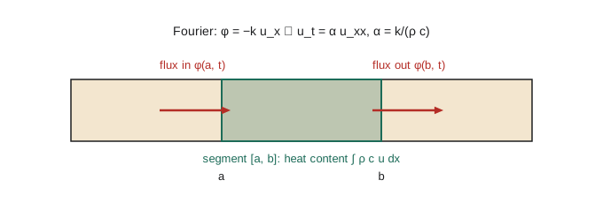
The heat energy in the segment \(a \le x \le b\) is \(\int_a^b \rho c\,u\,A\,dx\). Conservation of energy says its rate of change equals the heat flowing in at \(a\), minus the heat flowing out at \(b\), plus the heat produced inside:

after cancelling the common factor \(A\). By the fundamental theorem of calculus, \(\varphi(a, t) - \varphi(b, t) = -\int_a^b \varphi_x\,dx\). Bringing the time derivative inside the integral, which is legitimate when \(u_t\) is continuous, gives

for every interval \([a, b]\). If a continuous function has zero integral over every interval, it is identically zero: otherwise it would be positive (or negative) on some small interval around a point, and its integral there would be nonzero. So the integral form implies the local conservation law \(\rho c\,u_t + \varphi_x = Q\). The integral form is more fundamental, because it still makes sense when \(u\) has jumps, as at the interface between two materials.

Fourier's law and the heat equation

Conservation alone is one equation for two unknowns, \(u\) and \(\varphi\). The missing relation is a constitutive law describing the material. Fourier's law, based on experiment, says that heat flows from hot to cold at a rate proportional to the temperature gradient:

where \(k > 0\) is the thermal conductivity. The minus sign makes heat flow down the gradient. Substituting, with constant \(\rho\), \(c\) and \(k\), gives the heat equation with a source,

The thermal diffusivity \(\alpha\) has units of square metres per second. Typical values are \(1.1 \times 10^{-4}\) for copper, \(1.2 \times 10^{-5}\) for steel, \(1.4 \times 10^{-7}\) for water, \(8 \times 10^{-7}\) for granite and about \(10^{-6}\) for frozen soil. If the material properties vary with position, the derivation gives instead \(\rho c\,u_t = (k\,u_x)_x + Q\), the heat equation in divergence form, which is the right starting point for layered materials.

In three dimensions, the same argument applied to an arbitrary region \(V\) with boundary surface \(S\) and outward normal \(\mathbf n\) gives \(\frac{d}{dt}\iiint_V \rho c\,u\,dV = -\iint_S \boldsymbol\varphi\cdot\mathbf n\,dS + \iiint_V Q\,dV\). The divergence theorem turns the surface integral into \(\iiint_V \nabla\cdot\boldsymbol\varphi\,dV\), Fourier's law becomes \(\boldsymbol\varphi = -k\nabla u\), and the result is \(u_t = \alpha\Delta u + Q/(\rho c)\).

Boundary conditions from physics

The boundary conditions of lesson 1 now have physical meaning. A Dirichlet condition \(u(0, t) = T_0\) describes an end held at fixed temperature by contact with a large reservoir. A Neumann condition \(-k\,u_x(L, t) = \varphi_L\) prescribes the heat flux leaving the right end, with \(\varphi_L = 0\) for perfect insulation. A Robin condition \(-k\,u_x(L, t) = h\big(u(L, t) - u_a\big)\) describes an end that exchanges heat with surrounding air. The sign conventions matter: at the right end the outward normal points in the positive \(x\) direction, so outward flux is \(-k\,u_x\); at the left end it is \(+k\,u_x\). Getting this sign wrong turns a cooling condition into a heating one, and the resulting problem can have solutions that grow without bound.

The vibrating string

Now consider a perfectly flexible string stretched between two points, with linear density \(\rho\) (mass per unit length) and tension \(T\). Let \(u(x, t)\) be the small vertical displacement of the point at horizontal position \(x\). We assume that the motion is purely vertical, that the slope \(u_x\) is small, and that the tension is constant along the string. The string is flexible, so the force it exerts at any point is directed along its tangent.

Apply Newton's second law to the piece of string between \(x\) and \(x + \Delta x\). The vertical component of the tension at the right end is \(T\sin\theta(x + \Delta x)\), where \(\theta\) is the angle of the tangent with the horizontal; at the left end it is \(-T\sin\theta(x)\). For small slopes \(\sin\theta \approx \tan\theta = u_x\). The mass of the piece is approximately \(\rho\,\Delta x\), and its acceleration is \(u_{tt}\). So

Dividing by \(\Delta x\) and letting \(\Delta x \to 0\) gives the one-dimensional wave equation

The wave speed increases with tension and decreases with density, which is how a guitarist tunes a string. A steel guitar string with tension 70 N and density \(4 \times 10^{-3}\) kg/m has \(c \approx 132\) m/s. The horizontal force balance is consistent with constant tension, because \(T\cos\theta \approx T\) at both ends for small slopes. Adding gravity gives \(u_{tt} = c^2u_{xx} - g\); adding air resistance proportional to velocity gives the damped wave equation \(u_{tt} + \gamma u_t = c^2u_{xx}\), sometimes called the telegraph equation because it also describes signals on a long transmission line.

The same reasoning in two dimensions gives \(u_{tt} = c^2(u_{xx} + u_{yy})\) for a stretched membrane such as a drumhead, with \(c^2 = T/\rho\) now involving tension per unit length and mass per unit area. Sound waves follow from conservation of mass and momentum in a compressible gas: linearizing about rest gives the wave equation for the pressure perturbation, with \(c^2 = \gamma p_0/\rho_0\) for an ideal gas, about 343 m/s in air at 20 °C, as Laplace showed in 1816 by correcting Newton's isothermal estimate.

Steady states: Laplace and Poisson

If the boundary data and sources do not depend on time, the temperature in a body tends to a steady state with \(u_t = 0\). The heat equation then reduces to Poisson's equation \(-k\,\Delta u = Q\), and in a source-free region to Laplace's equation \(\Delta u = 0\). The same equation describes the shape of a membrane at rest under a load: \(-T\Delta u = f\). In electrostatics, Gauss's law \(\nabla\cdot\mathbf E = \rho_e/\varepsilon_0\) and \(\mathbf E = -\nabla V\) give \(\Delta V = -\rho_e/\varepsilon_0\). In ideal fluid flow, incompressibility \(\nabla\cdot\mathbf v = 0\) and irrotationality \(\mathbf v = \nabla\phi\) give \(\Delta\phi = 0\). In groundwater flow, Darcy's law \(\mathbf q = -K\nabla h\) and conservation of water give \(\Delta h = 0\) for the hydraulic head. One equation, four sciences.

Scaling and dimensionless variables

Physical constants can be removed by choosing natural units. For the heat equation on \(0 \le x \le L\), set \(x = L\xi\) and \(t = \tau\,s\) with \(\tau = L^2/\alpha\). Then \(u_t = u_s/\tau\) and \(u_{xx} = u_{\xi\xi}/L^2\), and the equation becomes \(u_s = u_{\xi\xi}\) on \(0 \le \xi \le 1\). The diffusion time \(L^2/\alpha\) is the single time scale of the problem. It grows with the square of the length: a copper rod 1 m long has \(\tau \approx 2.5\) hours, a 10 cm rod 90 seconds. A slab of granite 1 m thick takes about 15 days, and a 10 m depth of frozen ground about 3 years. For the wave equation the natural time scale is the transit time \(L/c\), proportional to length rather than its square, which is the dimensional signature of propagation versus diffusion.

Scaling reveals what can and cannot matter. In the dimensionless heat problem there are no parameters at all, so every insulated rod with fixed-temperature ends behaves the same way in its own units. With lateral cooling the single dimensionless group \(\beta L^2/\alpha\) appears and measures the strength of cooling against conduction. Engineers call such groups Biot or Fourier numbers.

Checking a derivation numerically

The program below takes a discretized rod, applies the conservation law cell by cell with Fourier's law for the fluxes between cells, and confirms that the total heat content changes exactly by the boundary fluxes. It then checks the steady state of the heated wire and the scaling of the diffusion time.

import math

# rod of length 1 m, steel: alpha = k/(rho c)
k, rho, c = 50.0, 7850.0, 490.0
alpha = k / (rho * c)
N, L = 50, 1.0
dx = L / N
u = [20.0 + 30.0 * math.sin(math.pi * (j + 0.5) * dx) for j in range(N)]   # cell averages
Tleft, Tright = 0.0, 100.0
dt = 0.4 * dx * dx / alpha

def fluxes(u):
    # phi = -k du/dx at each cell face; boundary faces use half-cell distance
    f = [-k * (u[0] - Tleft) / (dx / 2)]
    f += [-k * (u[j] - u[j - 1]) / dx for j in range(1, N)]
    f += [-k * (Tright - u[-1]) / (dx / 2)]
    return f

energy = lambda u: sum(rho * c * v * dx for v in u)
E0, net_in = energy(u), 0.0
for step in range(2000):
    f = fluxes(u)
    net_in += (f[0] - f[-1]) * dt
    u = [u[j] - dt / (rho * c) * (f[j + 1] - f[j]) / dx for j in range(N)]
print(f"alpha = {alpha:.3e} m^2/s, simulated {2000 * dt / 3600:.2f} h")
print(f"change in heat content {energy(u) - E0:.6e} J/m^2")
print(f"net heat through ends  {net_in:.6e} J/m^2")
xm = (N // 2 + 0.5) * dx
print(f"temperature at x = {xm:.2f}: {u[N // 2]:.2f} C, steady state there {Tleft + (Tright - Tleft) * xm:.2f} C")

# heated wire: steady state u = Q x (L - x) / (2k)
Q = 2.0e4
peak = Q * L * L / (8 * k)
print(f"heated wire peak temperature rise {peak:.1f} C; doubling L gives {4 * peak:.1f} C")

# diffusion times L^2/alpha
for name, a in (("copper", 1.1e-4), ("steel", alpha), ("granite", 8e-7), ("frozen soil", 1e-6)):
    for Lm in (0.1, 1.0, 10.0):
        T = Lm * Lm / a
        print(f"{name:12s} L = {Lm:5.1f} m: L^2/alpha = {T:12.0f} s = {T / 86400:9.2f} days")

alpha = 1.300e-05 m^2/s, simulated 6.84 h
change in heat content 4.106754e+07 J/m^2
net heat through ends  4.106754e+07 J/m^2
temperature at x = 0.51: 50.65 C, steady state there 51.00 C
heated wire peak temperature rise 50.0 C; doubling L gives 200.0 C
copper       L =   0.1 m: L^2/alpha =           91 s =      0.00 days
copper       L =   1.0 m: L^2/alpha =         9091 s =      0.11 days
copper       L =  10.0 m: L^2/alpha =       909091 s =     10.52 days
steel        L =   0.1 m: L^2/alpha =          769 s =      0.01 days
steel        L =   1.0 m: L^2/alpha =        76930 s =      0.89 days
steel        L =  10.0 m: L^2/alpha =      7693000 s =     89.04 days
granite      L =   0.1 m: L^2/alpha =        12500 s =      0.14 days
granite      L =   1.0 m: L^2/alpha =      1250000 s =     14.47 days
granite      L =  10.0 m: L^2/alpha =    125000000 s =   1446.76 days
frozen soil  L =   0.1 m: L^2/alpha =        10000 s =      0.12 days
frozen soil  L =   1.0 m: L^2/alpha =      1000000 s =     11.57 days
frozen soil  L =  10.0 m: L^2/alpha =    100000000 s =   1157.41 days

The change in heat content matches the net flux through the ends to rounding error, because each interior flux leaves one cell and enters its neighbour: the discrete scheme conserves energy exactly, as the integral form of the law demands. The diffusion table shows times spanning from seconds to years, all following \(L^2/\alpha\). After 6.8 hours, about a third of the steel rod's diffusion time of 21 hours, the midpoint is already within half a degree of its linear steady state. The reason is the factor \(\pi^2\) in the decay rate of the slowest mode, \(\pi^2\alpha/L^2\), which lesson 7 derives: over this run that mode shrinks by a factor of \(e^{-3.16} \approx 0.04\).