Fourier series

Fourier's great claim of 1807 was that any function on an interval, even one with corners and jumps, can be written as a sum of sines and cosines. That claim is what makes separation of variables work: if the initial temperature in a rod is a sum of sine waves, and each sine wave evolves in a simple known way under the heat equation, then the temperature at every later time is the corresponding sum of evolved waves. This lesson develops Fourier series on a symmetric interval: the orthogonality relations, the Euler–Fourier formulas for the coefficients, sine and cosine series on a half-interval, the complex form and Parseval's identity. The next lesson asks the delicate question of when and how the series converges.

Periodic functions and trigonometric series

A function \(f\) is periodic with period \(P\) if \(f(x + P) = f(x)\) for all \(x\). The functions \(\cos(n\pi x/L)\) and \(\sin(n\pi x/L)\) for \(n = 1, 2, 3, \ldots\) all have period \(2L\); the \(n\)-th one completes \(n\) oscillations over the interval \([-L, L]\). A trigonometric series is an expression of the form

If such a series converges, its sum has period \(2L\). The question is the reverse: given a function \(f\) on \([-L, L]\), can we find coefficients so that the series sums to \(f\), and if so, what are they? The term \(n = 1\) is called the fundamental and the others are harmonics, the language of music: a violin and a flute playing the same note have the same fundamental and different strengths of harmonics.

Orthogonality

The key to finding the coefficients is that the trigonometric functions are orthogonal on \([-L, L]\). For positive integers \(m\) and \(n\),

These follow from the product-to-sum identities. For example, \(\cos A\cos B = \frac12[\cos(A - B) + \cos(A + B)]\), and the integral of \(\cos(k\pi x/L)\) over a full period is zero for every nonzero integer \(k\), so only the case \(m = n\) survives, where \(\cos 0 = 1\) contributes \(\frac12 \cdot 2L = L\). The mixed integral vanishes because the integrand is odd. Also \(\int_{-L}^L 1\,dx = 2L\) and the integral of the constant against any \(\cos\) or \(\sin\) term is zero.

Orthogonality is a geometric idea. Define the inner product of two functions on \([-L, L]\) by \(\langle f, g\rangle = \int_{-L}^L f(x)g(x)\,dx\), the continuous analogue of the dot product \(\sum f_ig_i\). Then the functions \(1, \cos(\pi x/L), \sin(\pi x/L), \cos(2\pi x/L), \ldots\) are mutually perpendicular, like the coordinate axes of an infinite-dimensional space. Finding Fourier coefficients is finding the components of a vector along perpendicular axes, which is done by taking inner products.

The Euler–Fourier formulas

Suppose \(f(x) = \frac{a_0}{2} + \sum (a_n\cos(n\pi x/L) + b_n\sin(n\pi x/L))\) and that we may integrate term by term (true, for instance, when the series converges uniformly). Multiply both sides by \(\cos(m\pi x/L)\) and integrate over \([-L, L]\). By orthogonality every term vanishes except the one with \(n = m\), which gives \(La_m\). Doing the same with \(\sin(m\pi x/L)\) and with 1 gives the Euler–Fourier formulas

Writing the constant term as \(a_0/2\) lets one formula cover \(a_0\): it makes \(a_0/2\) the average value of \(f\) over the interval. For any integrable \(f\) these formulas define coefficients, and the resulting series is called the Fourier series of \(f\), written \(f \sim \frac{a_0}{2} + \sum(\cdots)\). The symbol \(\sim\) is deliberate. The formulas always make sense, but whether the series converges to \(f\) is a separate question, the subject of lesson 6. Euler had found these formulas in 1777 in a special case; Fourier was the first to assert that they apply to arbitrary functions.

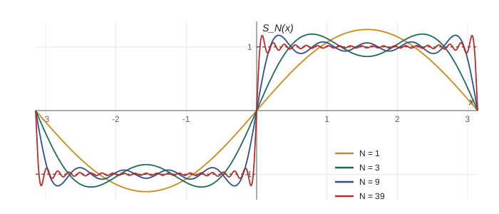
The figure shows the partial sums \(S_N(x) = \frac4\pi\sum_{n \le N,\,n \text{ odd}} \sin(nx)/n\). Away from the jumps at \(0\) and \(\pm\pi\) they converge to \(\pm1\). At the jumps every partial sum equals 0, the average of the values on either side. Next to the jumps there is an overshoot of about 9 hundredths of the jump size that never goes away: this is the Gibbs phenomenon of lesson 6. The coefficients decay like \(1/n\), slowly, because the function has jumps. Smoother functions have faster-decaying coefficients.

Even and odd functions; half-range series

A function is even if \(f(-x) = f(x)\) and odd if \(f(-x) = -f(x)\). The integral of an odd function over a symmetric interval is zero, and the integral of an even function is twice the integral over \([0, L]\). Since cosine is even and sine is odd, an even function has a pure cosine series and an odd function a pure sine series, with coefficients computed from \([0, L]\) alone.

This matters because PDE problems usually live on \([0, L]\), not on a symmetric interval. A function given only on \([0, L]\) can be extended to \([-L, L]\) in two natural ways. The odd extension, \(f(-x) = -f(x)\), produces the Fourier sine series; the even extension, \(f(-x) = f(x)\), produces the Fourier cosine series:

Both represent \(f\) on \((0, L)\), but they differ outside it and at the endpoints. Every sine term vanishes at \(0\) and \(L\), so the sine series suits Dirichlet conditions \(u(0) = u(L) = 0\). Every cosine term has zero derivative at \(0\) and \(L\), so the cosine series suits Neumann conditions. Lesson 7 shows that the boundary conditions choose the series automatically.

Complex form and Parseval's identity

Euler's formula \(e^{i\theta} = \cos\theta + i\sin\theta\) gives a compact form of the series. With \(\cos\theta = (e^{i\theta} + e^{-i\theta})/2\) and \(\sin\theta = (e^{i\theta} - e^{-i\theta})/(2i)\),

with \(c_n = (a_n - ib_n)/2\) and \(c_{-n} = \overline{c_n}\) for real \(f\). The complex exponentials are orthogonal with respect to the inner product \(\int f\bar g\,dx\). The complex form is the natural route to the Fourier transform, to the discrete Fourier transform of signal processing and to the fast Fourier transform algorithm.

Parseval's identity, named for Marc-Antoine Parseval, who stated a version of it in 1799, expresses the energy of a function through its coefficients, the infinite-dimensional Pythagorean theorem:

For the square wave the left side is \(\frac1\pi\cdot 2\pi = 2\), and the right side is \(\sum_{n \text{ odd}} 16/(n^2\pi^2)\), giving \(\sum_{n \text{ odd}} 1/n^2 = \pi^2/8\) once more, and from that \(\sum_{n \ge 1} 1/n^2 = \pi^2/6\), Euler's solution of the Basel problem. Parseval's identity also gives the error of truncation: the mean-square error of the partial sum \(S_N\) equals the sum of the squares of the omitted coefficients. Among all trigonometric polynomials of degree \(N\), the Fourier partial sum is the one that minimizes the mean-square error, which is the best-approximation property.

Computing coefficients numerically

For functions given by data or by formulas whose integrals are awkward, the coefficients can be computed by numerical integration. The program below uses composite Simpson's rule, splitting at the jump so that each piece is smooth, and checks the results for the square and triangle waves. It then measures the mean-square error of partial sums against Parseval's prediction and evaluates the partial sums at a few points.

import math

def simpson(g, a, b, n=2000):
    h = (b - a) / n
    s = g(a) + g(b)
    for i in range(1, n):
        s += (4 if i % 2 else 2) * g(a + i * h)
    return s * h / 3

def coeffs(f, N, L=math.pi, breaks=(0.0,)):
    pts = [-L] + list(breaks) + [L]
    eps = 1e-12                                # stay just inside each smooth piece
    integ = lambda g: sum(simpson(g, pts[i] + eps, pts[i + 1] - eps) for i in range(len(pts) - 1))
    a = [integ(lambda x: f(x) * math.cos(n * math.pi * x / L)) / L for n in range(N + 1)]
    b = [0.0] + [integ(lambda x: f(x) * math.sin(n * math.pi * x / L)) / L for n in range(1, N + 1)]
    return a, b

square = lambda x: 1.0 if x > 0 else -1.0
a, b = coeffs(square, 7)
print("square wave b_n:", " ".join(f"{(v if abs(v) > 5e-6 else 0.0):.5f}" for v in b[1:]))
print("exact 4/(n pi):  ", " ".join(f"{(4 / (n * math.pi) if n % 2 else 0):.5f}" for n in range(1, 8)))

tri = lambda x: abs(x)
a, b = coeffs(tri, 7)
print("|x| a_n:", " ".join(f"{abs(v) if abs(v) < 5e-6 else v:+.5f}" for v in a))

def S(x, a, b, L=math.pi):
    return a[0] / 2 + sum(a[n] * math.cos(n * x) + b[n] * math.sin(n * x) for n in range(1, len(a)))

# mean-square error of partial sums versus Parseval's prediction
a, b = coeffs(square, 101)
for N in (1, 5, 25, 101):
    M = 6000                                   # midpoint rule avoids the jump points
    err = 2 * math.pi / M * sum((1 - S((j + 0.5) * math.pi / M, a[:N + 1], b[:N + 1])) ** 2 for j in range(M))
    tail = math.pi * sum(16 / (n * n * math.pi ** 2) for n in range(N + 1, 200001) if n % 2)
    print(f"N = {N:3d}: integral of error^2 = {err:.5f}, sum of omitted coefficients^2 x pi = {tail:.5f}")

# partial sums at x = pi/2 approach 1 (Leibniz series)
for N in (1, 9, 99, 999):
    s = 4 / math.pi * sum((-1) ** ((n - 1) // 2) / n for n in range(1, N + 1, 2))
    print(f"S_{N}(pi/2) = {s:.6f}")

square wave b_n: 1.27324 0.00000 0.42441 0.00000 0.25465 0.00000 0.18189
exact 4/(n pi):   1.27324 0.00000 0.42441 0.00000 0.25465 0.00000 0.18189
|x| a_n: +3.14159 -1.27324 +0.00000 -0.14147 +0.00000 -0.05093 +0.00000 -0.02598
N =   1: integral of error^2 = 1.19023, sum of omitted coefficients^2 x pi = 1.19021
N =   5: integral of error^2 = 0.42062, sum of omitted coefficients^2 x pi = 0.42061
N =  25: integral of error^2 = 0.09789, sum of omitted coefficients^2 x pi = 0.09788
N = 101: integral of error^2 = 0.02496, sum of omitted coefficients^2 x pi = 0.02495
S_1(pi/2) = 1.273240
S_9(pi/2) = 1.063054
S_99(pi/2) = 0.993634
S_999(pi/2) = 0.999363

The computed coefficients agree with the exact ones to five or more decimal places, and the integrated squared error of each partial sum matches \(\pi\) times the sum of the squared omitted coefficients. Convergence at the point \(\pi/2\) is slow, with error roughly proportional to \(1/N\), because the coefficients themselves decay only like \(1/n\).

Why Fourier's claim was controversial

To eighteenth-century mathematicians a function was given by a single formula, and it seemed absurd that a sum of smooth, everywhere-analytic sines could equal a function defined by different formulas on different pieces, let alone one with jumps. Lagrange, who had met trigonometric series in his own work on strings, objected strongly to Fourier's 1807 memoir. Fourier's evidence was computational: he calculated coefficients, summed series, and checked against physical intuition. The prize memoir of 1812 and the 1822 book established the method; Dirichlet's theorem of 1829 gave the first rigorous convergence proof. In the process the very concept of a function was liberated from formulas, and the modern definition, an arbitrary rule assigning outputs to inputs, owes much to this debate.