
LES-203 · Lesson 10 of 12 · 25 min
Speed from tire marks and drag factor
▶ Video coming soon A video version of this lesson is on the way.
Three days after the collision, on a dry Tuesday morning with Kingsway closed for an hour, Kowalczyk drove a borrowed pickup of the same make, model and year as Halloran's along the westbound curb lane and braked as hard as he could at a cone. Constable Grace Teague, the unit's other reconstructionist, measured the stopping distance and checked the speed against a calibrated test unit. They did it again, and then a third time to check the first two. From those few metres of road, they would calculate the single most important number in the case: how fast Halloran's truck was travelling when its driver first hit the brakes.
This lesson explains the physics behind speed estimates from tire marks. It is the most mathematical lesson in the course, but every step uses one idea that most students already know: a moving vehicle that brakes hard slows down at a rate set by the grip between its tires and the road. If investigators know that rate and how far the vehicle slid, they can work out how fast it was going when the braking began.
Drag factor
The drag factor, written f, is the deceleration of a braking vehicle expressed as a fraction of the acceleration due to gravity. A drag factor of 0.72 means the vehicle slows at 0.72 times g, where g is about 9.81 metres per second squared. The drag factor depends on the road surface, its condition, the tires and the vehicle's brakes. It is closely related to the coefficient of friction between the tires and the road, and on a level road the two are usually treated as the same.
| Surface | Typical drag factor range |
|---|---|
| Dry asphalt, new or travelled | 0.65 to 0.90 |
| Wet asphalt | 0.45 to 0.75 |
| Dry concrete | 0.65 to 0.90 |
| Gravel, loose | 0.40 to 0.70 |
| Packed snow | 0.20 to 0.45 |
| Ice | 0.05 to 0.25 |
The ranges in the table are wide because surfaces vary so much. Investigators therefore do not rely on tables when they can measure. The best method is a test skid or test stop: a vehicle like the one involved, on the same stretch of road in the same conditions, braked hard from a known speed while its stopping distance is measured. Investigators may also use a drag sled, a weighted object with a tire tread surface pulled across the road with a force gauge, or an accelerometer in the test vehicle that measures the deceleration directly.
From physics to a formula
The formula comes from a basic equation of motion. A vehicle that slows from speed v to a stop at a constant deceleration a covers a distance d given by v squared equals 2 times a times d. Because the deceleration is the drag factor times g, the speed at the start of braking is the square root of 2 times f times g times d. Investigators usually use a version of this formula that gives the answer directly in the units they work with.
In metric units, with d in metres and the speed in kilometres per hour, the constant 2 times 9.81, multiplied by the square of 3.6 to convert metres per second to kilometres per hour, is about 254. The working formula is the square root of 254 times f times d.
Worked problem
Finding the drag factor from test stops
Kowalczyk's test pickup, with anti-lock brakes, stopped in 13.8 m and 13.5 m from 50 km/h. What drag factor do the tests give?
Show solution
- Rearrange the formula: f equals S squared divided by 254 times d.
- \[f_1 = \frac{50^2}{254 \times 13.8} = \frac{2500}{3505.2} \approx 0.713\]
- \[f_2 = \frac{2500}{254 \times 13.5} = \frac{2500}{3429} \approx 0.729\]
- The average of the two is about 0.72. The third test, used as a check, gave a result between them.
Answer: A drag factor of about 0.72 for that pickup on that road.
Teague points out why the test vehicle mattered. 'Anti-lock brakes stop a vehicle close to the peak grip of the tires, which is a little better than a fully locked skid on most dry surfaces. If we had tested with an old car without anti-lock brakes, we would have measured a lower drag factor and underestimated his speed. Testing with the same kind of truck gives the fairest number.'
Speed from marks to a stop
The simplest case is a vehicle that braked and slid to a stop without hitting anything. Then the formula gives its speed at the start of the marks directly. This is often used to check witness estimates and drivers' statements, and it is a common question on police training exams.
Worked problem
A skid to a stop on a wet road
A car leaves skid marks 30 m long on a wet asphalt road and stops without hitting anything. Test skids give a drag factor of 0.55. How fast was it going when the wheels locked?
Show solution
- \[S = \sqrt{254 \times 0.55 \times 30} = \sqrt{4191} \approx 64.7 \text{ km/h}\]
- This is the speed at the moment the marks began, not before. Any slowing before the wheels locked, and the driver's reaction time, are not included.
Answer: About 65 km/h.
Speed when the vehicle hit something
Halloran's truck did not slide to a stop; it was still moving when it struck the hatchback. The marks show only the speed it lost while braking, not all of its speed. If the impact speed is known, the speed at the start of braking can be found by combining the two. The energy at the start of the marks equals the energy lost in braking plus the energy left at impact, and because energy depends on the square of speed, the speeds combine as the square root of the sum of their squares.
If the impact speed is not known, investigators can still give a minimum speed: the speed the vehicle would have needed just to make the marks and stop. That is the speed lost in the marks alone, and because the truck was still moving at impact, its real speed must have been higher. Minimum speeds are valuable in court because they are conservative; they do not depend on any estimate of the impact.
Worked problem
The pickup's speed at the start of braking
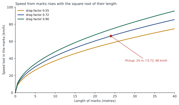
The pickup's anti-lock marks were 24.0 m long from their start to the point of impact, and the drag factor was 0.72. The truck's event data recorder, covered in lesson 11, and a momentum analysis both put its speed at impact at about 38 km/h. What was its speed at the start of braking, and what was its minimum speed from the marks alone?
Show solution
- Speed lost in the marks: 254 times 0.72 times 24.0 is 4,389.1.
- \[S_{\text{marks}} = \sqrt{4389.1} \approx 66.3 \text{ km/h}\]
- Add the square of the impact speed: 38 squared is 1,444.
- \[S_0 = \sqrt{1444 + 4389.1} = \sqrt{5833.1} \approx 76.4 \text{ km/h}\]
Answer: About 76 km/h at the start of braking, with a minimum of 66 km/h from the marks alone, in a 50 km/h zone.
Uncertainty and ranges
Every measurement has some uncertainty, and investigators show the effect of that uncertainty on their conclusions. The usual approach is to calculate a range using the lowest and highest reasonable values of each input. If even the lowest value supports the conclusion, the conclusion is strong. In court, a reconstructionist who gives a range, and explains how it was calculated, is far more persuasive than one who gives a single number with false precision.
| Drag factor | Speed lost in 24.0 m | With 38 km/h at impact |
|---|---|---|
| 0.70 | 65.3 km/h | 75.6 km/h |
| 0.72 | 66.3 km/h | 76.4 km/h |
| 0.75 | 67.6 km/h | 77.6 km/h |
Kowalczyk's report gave the pickup's speed at the start of braking as 75 to 78 km/h, and at least 65 km/h from the marks alone. The posted limit was 50 km/h. Even the most conservative figure, the minimum from the marks alone with the lowest drag factor, was well over the limit, and that was before allowing for any slowing before the anti-lock system engaged. Teague notes how this matched Coutu's lidar reading of 81 km/h fifty-three minutes earlier, less than two kilometres away. 'Two independent methods, one an hour apart, both say the same thing about how he was driving that night.'
Grades and changes in surface
Two adjustments are common. On a hill, gravity helps or hinders the braking. On an uphill grade, the effective drag factor is the measured drag factor plus the grade, written as a decimal; on a downhill grade, the grade is subtracted. A downgrade of 5 in 100 reduces a drag factor of 0.72 to about 0.67. Kingsway is nearly level at the collision site, so no adjustment was needed.
When a vehicle slides across two surfaces, such as from asphalt onto a gravel shoulder, each section is calculated separately and the results combined, again by adding the squares. The combined formula is the square root of the constant times the sum of each drag factor multiplied by its distance.
Worked problem
Marks across two surfaces
A car skids 12 m on dry asphalt, with a drag factor of 0.72, and then 8 m on a gravel shoulder, with a drag factor of 0.50, before stopping. How fast was it going at the start of the marks?
Show solution
- Multiply each drag factor by its distance and add: 0.72 times 12 is 8.64, and 0.50 times 8 is 4.00, for a total of 12.64.
- \[S = \sqrt{254 \times 12.64} = \sqrt{3210.6} \approx 56.7 \text{ km/h}\]
Answer: About 57 km/h.
Limits of the method
Speed from marks is reliable when the inputs are reliable, and investigators are careful about its limits. The marks must belong to the vehicle in question, which is why tire widths, positions and patterns are measured. All the tires that braked must be accounted for; a vehicle braking on only some wheels, because of a defect or a trailer, has a lower drag factor. The marks show the speed only from the point where they begin, so any slowing before they start, during the driver's reaction or before the anti-lock system engaged, is not included, which again makes the estimate conservative. And anti-lock marks can fade so that their true start is hard to see, which is why Kowalczyk's careful search for the faint start of the left front mark mattered: the 1.5 metres he found added nearly two kilometres an hour to the final estimate.
Desjardins closes the lesson with a reminder about the purpose of the arithmetic. 'Rosa Pereira's family will not care about square roots. They will care whether the man who hit their mother was speeding. The square roots are how we answer that honestly, with a number that can be checked by anyone who doubts it.'
Checking the arithmetic
Reconstructionists check every result against common sense before they rely on it. A speed that seems far too high or too low usually signals an error in a unit conversion, a misread measurement or the wrong formula. Teague's habit is to compare each answer with something she knows: a car at 50 km/h needs roughly 14 metres to stop on dry asphalt once the brakes are on, and one at 100 km/h needs roughly four times as far. If a calculation does not fit those landmarks, she looks for the mistake before writing a word of the report.
Common mistakes
MistakeThe marks show the vehicle's full speed.
InsteadThey show the speed lost while braking; if the vehicle hit something, its impact speed must be added by squares.
MistakeDrag factors should be taken from a table.
InsteadTables give wide ranges; test stops with a similar vehicle on the same road are better.
MistakeDoubling the length of the marks doubles the speed.
InsteadSpeed rises with the square root of the length, so doubling the length raises the speed by about 1.4 times.
MistakeA single precise number is more convincing in court.
InsteadA range calculated from reasonable inputs is more honest and more persuasive.
Summary and key terms
- The drag factor is the braking deceleration as a fraction of g.
- The working formula is S equals the square root of 254 f d, in km/h and metres.
- Test stops with a similar vehicle on the same road give the most reliable drag factor.
- When a vehicle hits something, its starting speed is the square root of the impact speed squared plus the speed lost in the marks squared.
- Minimum speeds and ranges make estimates conservative and defensible.
- Grades change the effective drag factor, and different surfaces are combined by adding their contributions.
- Drag factor
- The deceleration of a braking vehicle as a fraction of the acceleration due to gravity.
- Test stop
- A controlled hard stop with a similar vehicle used to measure the drag factor.
- Minimum speed
- The speed a vehicle needed just to leave the measured marks, ignoring any speed it still had at impact.
- Grade
- The slope of a road, expressed as the rise divided by the run.
Practice problems
Work each problem on paper first, then reveal the answer to check.
What does a drag factor of 0.72 mean?
Show answer
That the braking vehicle slows at 0.72 times the acceleration due to gravity.
Why did Kowalczyk test with a pickup like Halloran's?
Show answer
Because anti-lock brakes and the vehicle type affect the drag factor, and a similar vehicle gives the fairest value.
How are the impact speed and the speed lost in the marks combined?
Show answer
By taking the square root of the sum of their squares.
Why are speed-from-marks estimates usually conservative?
Show answer
Because they do not include any slowing before the marks began.
Lesson quiz · 5 questions
Score 60% or more to complete this lesson.
Create a free account to save your progress, take quizzes and earn a certificate.