
GEOM-499 · Lesson 6 of 12 · 22 min
Processing and adjustment
Processing turns raw observations into coordinates, surfaces and images that can be trusted. In the capstone it is where most of the hours go and where most of the hidden problems appear. The order matters. Control comes first, because every other product is fixed to it. Then the slope targets, the photogrammetric block, the scans and finally the terrain models and orthomosaic. At each step the team asks two questions: did the adjustment fit the observations as well as expected, and are the results consistent with independent checks? This lesson follows epoch 1 through that sequence and shows how least squares adjustment answers the first question.
Why least squares
Every survey in this project has more observations than unknowns. Six control marks are tied to CR1 by more baselines than strictly needed; the levelling loop has seven height differences for four unknown heights; the drone block has thousands of image measurements for a few hundred camera and point parameters. Redundant observations disagree slightly because of random errors. Least squares finds the set of unknowns that makes the weighted sum of the squared residuals as small as possible, and it also gives the precision of each unknown and statistics that show whether the observations behaved as expected.
Here A is the design matrix linking observations to unknowns, P is the weight matrix, the inverse of the observation variances, l holds the observations corrected for known values, v are the residuals, n is the number of observations and u the number of unknowns. The a posteriori variance factor sigma zero squared should be close to one if the weights were realistic. A value much larger than one means the observations are worse than assumed or contain a blunder; a value much smaller than one means the weights were too pessimistic.
GNSS baseline processing and the network adjustment
Jonas processes the static sessions with the precise orbits and clocks from the international GNSS service, which are available a couple of weeks after observation, and with the antenna calibrations for each antenna type. Each session yields a set of baselines with their covariance matrices. He first runs a minimally constrained adjustment, holding only CR1 fixed. This tests the internal consistency of the observations without letting errors in the datum hide them. The variance factor is close to one, and no baseline residual exceeds three times its standard deviation, but one baseline from session A at CW3, the mark with the obstructed eastern sky, has the largest normalized residual. The session B baseline at CW3 agrees well with the rest.
Next he runs the constrained adjustment, holding CR1 at its published coordinates and checking against the second reference station. The coordinates of the six marks change by a few millimetres from the minimally constrained solution, which shows that the datum and the network fit each other. The 95 percent relative error ellipses between neighbouring marks have semi-major axes of 3 to 6 mm horizontally and 8 to 12 mm vertically, well inside requirement R1.
The levelling network
The levelling loop gives the heights the canal engineers asked for. It has seven measured height differences connecting CR1 and four marks, so three degrees of freedom remain after solving for four heights. Each observation is weighted by the inverse of its variance, assuming 1.0 mm per root kilometre. The script builds the design matrix, solves the normal equations with the small matrix toolkit used in the earlier courses, and tests the result.
# Coulee Watch: least-squares adjustment of the epoch 1 height loop
import math
def T(A): return [list(r) for r in zip(*A)]
def mul(A, B): return [[sum(a * b for a, b in zip(r, c)) for c in zip(*B)] for r in A]
def inv(A):
    n = len(A); M = [list(map(float, r)) + [1.0 if i == j else 0.0 for j in range(n)] for i, r in enumerate(A)]
    for c in range(n):
        p = max(range(c, n), key=lambda r: abs(M[r][c])); M[c], M[p] = M[p], M[c]
        d = M[c][c]; M[c] = [x / d for x in M[c]]
        for r in range(n):
            if r != c:
                f = M[r][c]; M[r] = [x - f * y for x, y in zip(M[r], M[c])]
    return [r[n:] for r in M]
def diag(v): return [[v[i] if i == j else 0.0 for j in range(len(v))] for i in range(len(v))]
def col(v): return [[x] for x in v]
H_CR1 = 900.0 + 12.874        # fixed height of CR1 (m)
# observed height differences: from, to, dh (m), length (km)
obs = [("CR1", "CW1", -3.4154, 0.42), ("CW1", "CW2", -18.2281, 0.61),
       ("CW2", "CW3", -21.9021, 0.55), ("CW3", "CW4", 1.2202, 0.48),
       ("CW4", "CR1", 42.3264, 1.10), ("CW1", "CW4", -38.9102, 0.95),
       ("CW2", "CW4", -20.6813, 0.70)]
names = ["CW1", "CW2", "CW3", "CW4"]
A, l, w = [], [], []
for a, b, dh, km in obs:
    row = [0.0] * 4
    if a in names: row[names.index(a)] -= 1
    if b in names: row[names.index(b)] += 1
    c = dh + (H_CR1 if a == "CR1" else 0) - (H_CR1 if b == "CR1" else 0)
    A.append(row); l.append(c); w.append(1 / (0.0010 ** 2 * km))   # 1.0 mm per root km
P = diag(w)
N = mul(mul(T(A), P), A); x = mul(inv(N), mul(mul(T(A), P), col(l)))
v = [sum(A[i][j] * x[j][0] for j in range(4)) - l[i] for i in range(len(l))]
dof = len(l) - 4
s0sq = sum(w[i] * v[i] ** 2 for i in range(len(v))) / dof
Qx = inv(N)
for j, n in enumerate(names):
    print(f"{n}  H = {x[j][0]:9.4f} m   sigma = {math.sqrt(s0sq * Qx[j][j]) * 1000:4.1f} mm")
for (a, b, dh, km), r in zip(obs, v):
    print(f"{a}-{b}  residual {r * 1000:+5.1f} mm")
# global test: chi-square on dof, bounds by the Wilson-Hilferty approximation
def chi2q(p, k):
    z = {0.025: -1.95996, 0.975: 1.95996}[p]
    return k * (1 - 2 / (9 * k) + z * math.sqrt(2 / (9 * k))) ** 3
stat = dof * s0sq
print(f"variance factor {s0sq:.2f}, test statistic {stat:.2f} on {dof} dof, "
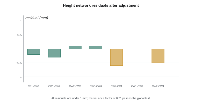
f"bounds {chi2q(0.025, dof):.2f} to {chi2q(0.975, dof):.2f}")CW1 H = 909.4584 m sigma = 0.3 mm CW2 H = 891.2299 m sigma = 0.4 mm CW3 H = 869.3279 m sigma = 0.5 mm CW4 H = 870.5482 m sigma = 0.4 mm CR1-CW1 residual -0.2 mm CW1-CW2 residual -0.3 mm CW2-CW3 residual +0.1 mm CW3-CW4 residual +0.1 mm CW4-CR1 residual -0.6 mm CW1-CW4 residual +0.0 mm CW2-CW4 residual -0.5 mm variance factor 0.31, test statistic 0.93 on 3 dof, bounds 0.18 to 9.32
The adjusted heights have standard deviations of 0.3 to 0.5 mm, and all residuals are below 1 mm. The variance factor is 0.31. The global test compares the statistic, the degrees of freedom times the variance factor, with the 2.5 and 97.5 percent points of the chi-square distribution for three degrees of freedom, roughly 0.2 and 9.3. The value of 0.93 lies inside, so the test passes. A variance factor below one simply suggests the levelling was a little better than the 1 mm per root kilometre assumed; with only three degrees of freedom the estimate is itself uncertain, so the team keeps the original weighting.
The levelled heights of CW1 to CW4 agree with the GNSS heights from the constrained adjustment to within 6 mm once the geoid model is applied. That agreement is an independent check on both the geoid model over this small area and the GNSS heights, and it is reported. Where both are available, the levelled heights are used for the foot marks.
Worked problem
Weights for a levelling line
A levelling line of 0.64 km is observed with a standard deviation of 1.0 mm per root kilometre. What is its standard deviation and its weight in units of mm to the minus two?
Show solution
- \[\sigma = 1.0\sqrt{0.64} = 0.80 \text{ mm}\]
- \[w = \frac{1}{\sigma^2} = \frac{1}{0.64} = 1.56 \text{ mm}^{-2}\]
Answer: The line has a standard deviation of 0.8 mm and a weight of 1.56. Longer lines get smaller weights, so short, precise lines dominate the solution.
Slope targets
The total station observations to the slope targets are adjusted as a small network with the control marks CW2 and CW4 fixed. Each target is observed from two marks with two sets, so its position is overdetermined. The standard deviations come out at about 3 to 4 mm per axis, as planned, except for the two upper targets partly hidden by shrubs, which reach 5 mm. These precisions feed the movement test in lesson 7. An adjustment with a variance factor near one and no flagged residuals means the targets were set and observed consistently.
The photogrammetric block
Sofia processes the drone images in photogrammetric software that runs structure from motion followed by a bundle adjustment, as covered in the photogrammetry course. She starts with only the image positions from the drone's onboard GNSS, which gives a block that is internally consistent but shifted and slightly bent. She then marks the 14 control targets in the images and runs the bundle adjustment again with the targets as control. The camera is self-calibrated in the adjustment, solving for focal length, principal point and lens distortion, because the oblique pass and the large height range on the slope make those parameters well determined.
The bundle adjustment report is checked line by line. The mean reprojection error is about 0.6 pixels, normal for this camera. The control targets fit with residuals of 1 to 2 cm horizontally and 1.5 to 3 cm vertically. One target on the lower bench shows a vertical residual of 6 cm; when Sofia looks at the images she finds that she marked the corner of the target rather than its centre in four images. After correcting the marks the residual drops to 2 cm. Without the check, that error would have tilted the lower slope of the model by a few centimetres.
The 32 checkpoints are not used in the adjustment. They are only measured in the images after processing is complete, for the accuracy assessment in lesson 8. Keeping them out of the adjustment is the only way they can test it.
Scan registration and georeferencing
Liam registers the four scans using the spherical targets and refines the registration with a cloud-to-cloud adjustment of the overlapping areas. The root mean square of target residuals is 3 mm and the cloud-to-cloud fit about 4 mm. The registered point cloud is then georeferenced to the control network through the spherical targets that were also measured from the control marks. The georeferencing residuals are 4 to 6 mm. The scan cloud and the photogrammetric cloud are compared on the overlapping bare toe: they agree with a mean vertical difference of 1.2 cm and a standard deviation of 2.1 cm, consistent with the expected accuracy of the drone model.
Terrain models and the orthomosaic
From the bundle adjustment, dense matching produces a point cloud of about 350 points per square metre. Ground filtering removes vegetation and other objects, using a cloth-simulation filter tuned on the slope and checked against the scan cloud. The filtered ground points are combined with the scan points on the toe, where the scans take precedence, and gridded to a terrain model with 10 cm cells. The orthomosaic is produced at 2.5 cm from the nadir images rectified onto a surface model. Both products are delivered in the project frame with the metadata described in lesson 11.
| Product | Main processing step | Internal check | Result |
|---|---|---|---|
| Control network | Baseline processing and network adjustment | Variance factor, residuals, second reference station | Passes; 95 % relative ellipses 3 to 6 mm |
| Levelling | Weighted least squares | Chi-square global test | Passes; heights to 0.3 to 0.5 mm |
| Slope targets | Total station network adjustment | Residuals, two stations | 3 to 5 mm per axis |
| Drone block | Bundle adjustment with self-calibration | Control residuals, reprojection error | One marking error found and fixed |
| Scans | Target and cloud-to-cloud registration | Target residuals, comparison with drone cloud | 3 to 6 mm; 1.2 cm bias to drone cloud |
Documenting the processing
Every processing run is recorded: the software and version, the settings, the inputs, the outputs and the summary statistics. The team keeps these records in a processing log that sits beside the data. When the second epoch is processed in April, the same software versions and settings are used, and any unavoidable change is noted. This matters because a change in a processing setting, such as the ground filter parameters, can produce a difference between epochs that has nothing to do with the ground.
Common mistakes
MistakeFixing every control point in the first adjustment.
InsteadRun a minimally constrained adjustment first to test the observations, then constrain to the datum.
MistakeChanging weights until the variance factor equals one.
InsteadInvestigate the cause; with few degrees of freedom the variance factor is itself uncertain.
MistakeUsing checkpoints as control in the bundle adjustment.
InsteadMeasure checkpoints only after processing so they remain independent tests.
MistakeUsing different software settings in the second epoch.
InsteadKeep processing settings constant between epochs, or apparent change may be a processing artifact.
Summary and key terms
- Least squares gives the best fit to redundant observations, precision estimates and quality statistics.
- A minimally constrained adjustment tests the observations; a constrained one ties them to the datum.
- The variance factor and chi-square global test check whether the observations fit their assumed precision.
- Bundle adjustment with self-calibration fixes the drone block to control; residuals reveal marking errors.
- Scans are registered by targets and cloud-to-cloud fitting and compared with the drone surface on overlap.
- A processing log with software, versions and settings lets the second epoch be processed identically.
- Least squares
- An adjustment that minimizes the weighted sum of squared residuals of redundant observations.
- Variance factor
- The a posteriori estimate of the reference variance; near one when weights are realistic.
- Global test
- A chi-square test of whether the variance factor is consistent with its expected value.
- Minimally constrained adjustment
- An adjustment holding only enough to define the datum, used to test observations.
- Self-calibration
- Solving for camera interior parameters within the bundle adjustment.
- Cloud-to-cloud registration
- Aligning point clouds by minimizing distances between their overlapping surfaces.
Practice problems
Work each problem on paper first, then reveal the answer to check.
A levelling network has 9 observations and 5 unknown heights. How many degrees of freedom are there?
Show answer
Four.
The variance factor is 3.8 with 10 degrees of freedom. What does that suggest?
Show answer
The observations are worse than assumed or contain a blunder; investigate residuals.
Why are checkpoints measured only after the bundle adjustment?
Show answer
So that they remain independent tests of the result.
What independent check confirmed the GNSS heights at the foot marks?
Show answer
Agreement with the levelled heights within 6 mm after applying the geoid model.
What error caused a 6 cm residual at one control target?
Show answer
The target corner instead of its centre was marked in four images.
Why are the scans given precedence on the toe?
Show answer
They are more accurate and see the steep toe better than the drone images.
Lesson quiz · 5 questions
Score 60% or more to complete this lesson.
Create a free account to save your progress, take quizzes and earn a certificate.