
GEOM-430 · Lesson 8 of 12 · 20 min
Crustal deformation
Lesson 3 treated plates as rigid. Near their edges they are anything but. The crust stretches, shortens and shears, faults lock and slip, and the ground deforms slowly for years before and after earthquakes. Measuring this deformation is one of geodesy's great contributions to the Earth sciences and to public safety, and it is done with the same instruments surveyors use every day, applied with extraordinary care. This lesson explains how velocities are turned into strain, how the earthquake cycle appears in geodetic data, and how these signals affect coordinates and frames.
For Coulee Geomatics, the subject arrives in two ways. The university group is studying how the reservoir bends the crust near the dam, a tiny deformation. And Leah has been asked by a former classmate at a Vancouver firm to review a strain-rate analysis on Vancouver Island, where the deformation is anything but tiny.
From velocities to strain
Strain is the change of shape of a body, expressed as relative changes of length and angle. In geodesy it is computed from how velocities vary from place to place. Within a small region, velocities can be approximated by a linear function of position, whose gradient tensor contains everything about the deformation. Its symmetric part is the strain rate tensor; its antisymmetric part is the rotation rate.
With three stations forming a triangle, the gradient is determined exactly; with more, it is estimated by least squares and its uncertainty can be judged. The principal strain rates, found from the eigenvalues of the tensor, show the directions of greatest stretching and shortening. Strain rates are tiny numbers: a velocity difference of 1 mm per year over 100 km is 10 nanostrain, or 10 parts per billion, per year. Geodesists usually quote them in nanostrain per year.
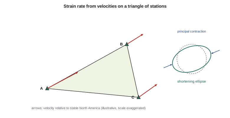
The code computes the strain rate from three illustrative stations on Vancouver Island, with velocities relative to stable North America, then shows an interseismic velocity profile across a locked strike-slip fault.
import math
# Strain rate from three GNSS stations (velocity gradient on a triangle), plus a 2D interseismic profile.
# Station positions (km east, km north) and velocities relative to stable North America (mm/yr), illustrative
P = [("UCLU", 0, 0, 7.5, 4.0), ("NANO", 110, 60, 4.0, 2.5), ("VICT", 120, -40, 4.5, 3.2)]
# Fit v = v0 + G * x for each component; three stations give an exact solution
def solve3(A, y):
    import copy
    M = [row[:] + [v] for row, v in zip(copy.deepcopy(A), y)]
    for c in range(3):
        p = max(range(c, 3), key=lambda r: abs(M[r][c])); M[c], M[p] = M[p], M[c]
        for r in range(3):
            if r != c:
                f = M[r][c] / M[c][c]; M[r] = [a - f * b for a, b in zip(M[r], M[c])]
    return [M[i][3] / M[i][i] for i in range(3)]
A = [[1.0, x, y] for _, x, y, _, _ in P]
ae = solve3(A, [ve for *_, ve, _ in P]); an = solve3(A, [vn for *_, vn in P])
dvedx, dvedy, dvndx, dvndy = ae[1], ae[2], an[1], an[2]     # mm/yr per km = 1e-6 per yr (microstrain/yr)
exx, eyy, exy = dvedx, dvndy, 0.5 * (dvedy + dvndx)
rot = 0.5 * (dvndx - dvedy)
avg = 0.5 * (exx + eyy); rad = math.sqrt((0.5 * (exx - eyy)) ** 2 + exy ** 2)
e1, e2 = avg + rad, avg - rad
theta = 0.5 * math.degrees(math.atan2(2 * exy, exx - eyy))
az1 = (90 - theta) % 180
print(f"exx {exx * 1000:+.1f}  eyy {eyy * 1000:+.1f}  exy {exy * 1000:+.1f} nanostrain/yr")
print(f"principal: e1 {e1 * 1000:+.1f} (azimuth {az1:.0f}), e2 {e2 * 1000:+.1f} nanostrain/yr")
print(f"rotation {rot * 1000:+.1f} nanoradian/yr (positive anticlockwise)")
print(f"dilatation {(exx + eyy) * 1000:+.1f} nanostrain/yr")
# Interseismic profile across a locked strike-slip fault: v(x) = (s / pi) * atan(x / D)
s, D = 30.0, 15.0     # slip rate mm/yr, locking depth km (illustrative)
for x in (-60, -20, -5, 0, 5, 20, 60):
print(f"x = {x:+4d} km v = {s / math.pi * math.atan(x / D):+6.2f} mm/yr")exx -27.6 eyy -7.9 exy -8.5 nanostrain/yr principal: e1 -4.7 (azimuth 160), e2 -30.8 nanostrain/yr rotation -0.8 nanoradian/yr (positive anticlockwise) dilatation -35.5 nanostrain/yr x = -60 km v = -12.66 mm/yr x = -20 km v = -8.86 mm/yr x = -5 km v = -3.07 mm/yr x = +0 km v = +0.00 mm/yr x = +5 km v = +3.07 mm/yr x = +20 km v = +8.86 mm/yr x = +60 km v = +12.66 mm/yr
The triangle is shortening: the principal strain rate e₂ is about −31 nanostrain per year, along an axis at azimuth 70°, roughly east-north-east, which is the direction in which the Juan de Fuca plate converges with North America. The other principal rate is small, −5 nanostrain per year, and the rotation is nearly zero. Dilatation, the sum of the normal strains, is about −36 nanostrain per year, meaning the area of the triangle shrinks. All of this is what one expects above a locked subduction zone, where the coast is being squeezed elastically as the plates stick.
How reliable is a strain rate?
Strain rates are derivatives, and derivatives amplify noise. If each velocity has an uncertainty of 0.3 mm per year and the stations are 100 km apart, the strain rate is uncertain by several nanostrain per year, which can be as large as the signal in a stable region. For a triangle with sides of 10 km the uncertainty is ten times larger. Analysts therefore prefer many stations and least squares over exact triangles, and they look at the uncertainty ellipse of each principal axis before interpreting directions. They also check that the velocities are in a consistent frame and from records of similar length, since mixing campaign and continuous stations, or velocities from different processing, can create spurious strain.
Rigid motion of the whole region, whether plate rotation or a frame error that rotates or translates everything, adds nothing to the strain. This is why strain is a robust quantity: it does not depend on the choice of frame in the way velocities do. But a frame scale rate, or an error that varies with position, such as an uncorrected antenna model affecting some stations and not others, does create strain. A careful analysis reports the strain together with the residual velocities after the fit, so that a reader can see whether a single station dominates the result.
The earthquake cycle
Faults do not slip steadily near the surface. For decades or centuries they stay locked while the plates continue to move, and the crust around them bends elastically, storing strain. In an earthquake the fault slips suddenly by metres, releasing the strain, and the ground near the fault jumps. Afterwards, the ground keeps moving for years as the deeper parts of the fault creep and the hot mantle flows. Geodesy sees all three phases: interseismic, coseismic and postseismic.
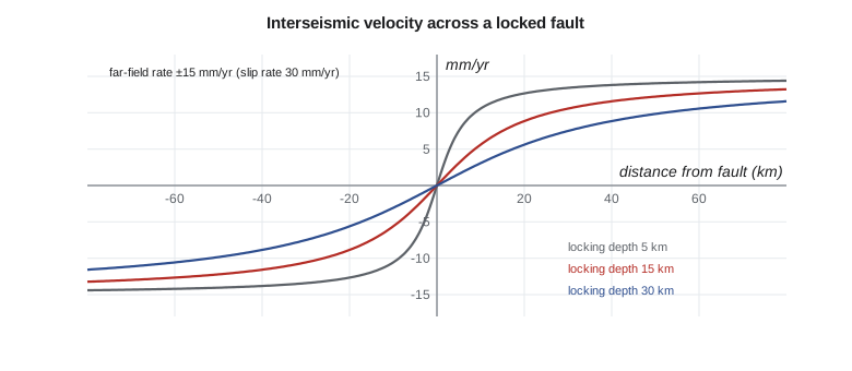
For a long, straight strike-slip fault locked to depth D and slipping freely below at rate s, the interseismic velocity parallel to the fault varies across it as an arctangent, a classic result due to Savage and Burford in 1973. The profile in the code, with s = 30 mm per year and D = 15 km, changes most quickly within about 20 km of the fault and reaches nearly ±15 mm per year at 60 km. By fitting such a profile to GNSS velocities, geodesists estimate both the slip rate and the locking depth, which together tell how fast strain is accumulating for the next earthquake.
Subduction zones are more complicated because the interface dips and the plates converge rather than slide past. At Cascadia, the plate interface is thought to be locked offshore, and GNSS stations on the coast move landward and upward, while those further inland move less. The region has not had a great earthquake since January 1700, a date known from Japanese records of the tsunami it caused and from tree rings in drowned coastal forests. Geodetic measurements of the accumulating strain are a central input to seismic hazard estimates for Victoria, Vancouver, Seattle and Portland.
A remarkable discovery of the early 2000s, first identified with GNSS on Vancouver Island and in Washington, is episodic tremor and slip. Every year or so in northern Cascadia, the deep part of the plate interface slips slowly over a couple of weeks, moving stations a few millimetres seaward, reversing their usual landward motion, accompanied by faint seismic tremor. These slow slip events release some strain without earthquakes and may load the locked zone above. They were invisible to seismometers until continuous GNSS showed the pattern.
Coseismic and postseismic motion
A large earthquake moves stations by centimetres to metres, sometimes hundreds of kilometres from the epicentre. The 2011 Tohoku earthquake in Japan moved parts of the coast by more than 5 m horizontally and lowered it by about a metre, and its slow postseismic motion continues. The 2016 Kaikoura earthquake in New Zealand, the 2010 Maule earthquake in Chile and the 2004 Sumatra earthquake had similar effects. Such jumps are discontinuities in station trajectories, and postseismic motion is non-linear: often a logarithmic or exponential decay over years. Since ITRF2014, the frame has included parametric models of postseismic deformation at affected stations, which is the only way to give them coordinates that remain valid.
For national frames, a great earthquake is a practical crisis. After the 1964 Alaska earthquake, the largest in North American history, large areas of land moved metres, and later surveys had to be adjusted. Countries on plate boundaries, such as New Zealand and Japan, now build deformation models into their national frames so that coordinates can be updated after an event. Canada and the United States are preparing for the same need on the west coast.
Other deformation
| Source | Typical signal | Measured by |
|---|---|---|
| Glacial isostatic adjustment | Up to 1 cm/yr up, mm/yr horizontal | GNSS, absolute gravity, GRACE |
| Volcanic inflation | Centimetres to metres over months | GNSS, InSAR, tiltmeters |
| Groundwater pumping | Up to tens of cm/yr down locally | InSAR, GNSS, levelling |
| Reservoir and lake loading | Millimetres, seasonal | GNSS, levelling |
| Landslides and slope creep | Centimetres to metres per year | GNSS, InSAR, monitoring surveys |
Interferometric synthetic aperture radar, introduced in GEOM-320, complements GNSS by mapping deformation over whole regions at once, though only in the satellite's line of sight and relative to a reference area. GNSS provides the frame for InSAR and the three-dimensional motion at points, and InSAR fills in the space between stations. Combining the two is standard for mapping subsidence from groundwater pumping, for which InSAR has revealed rates of tens of centimetres per year in parts of California's Central Valley, and for monitoring volcanoes and landslides.
Deformation also matters to surveyors in a direct, practical way. In a region straining at 40 nanostrain per year, a 10 km baseline changes length by 0.4 mm per year, or 4 mm per decade. That is negligible for most work but not for control networks used over many years, for monitoring structures that span faults, or for comparing old and new surveys. Agencies in deforming regions publish velocity models so that surveys made at different epochs can be compared, which lesson 9 takes up.
The district's tiny strain
Back at the dam, the university group wants to know whether the spring rise of the reservoir strains the crust measurably. Theo computes the strain between the three dam monitoring pillars and CR1 from their monthly positions, using the same method as the code. The answer is no signal above the noise: the expected elastic strain from a few metres of water over a few square kilometres is a few nanostrain at most, far below what monthly total station and GNSS measurements over a few hundred metres can detect. The vertical signal at CR1 is a better target, as lesson 5 suggested. Ruth is not disappointed. A clearly reported non-detection, with its limits, is a useful result.
Worked problem
Strain from two stations
Two stations 50 km apart along an east-west line have east velocities of 4.2 and 3.7 mm per year. What is the east-west strain rate?
Show solution
- \[\dot{\varepsilon}_{xx} = \frac{3.7 - 4.2}{50\ \text{km}} = \frac{-0.5\ \text{mm/yr}}{50\,000\ \text{m}} = -1.0 \times 10^{-8}\ \text{per yr}\]
Answer: About −10 nanostrain per year: shortening.
Common mistakes
MistakeUsing velocities in a global frame to compute strain without care.
InsteadRigid rotation does not change strain, but frame errors and noise do; check the residuals.
MistakeTreating a coseismic jump as part of the linear velocity.
InsteadModel offsets and postseismic decay separately.
MistakeInterpreting strain from a triangle with very short sides.
InsteadShort sides magnify noise; use well-spread stations.
MistakeAssuming slow slip events are noise.
InsteadThey are real, recurring signals in northern Cascadia.
Summary and key terms
- Strain rates come from the spatial gradient of velocities; rotation is its antisymmetric part.
- Geodetic strain rates are quoted in nanostrain per year.
- The earthquake cycle has interseismic, coseismic and postseismic phases.
- An arctangent profile describes interseismic motion across a locked strike-slip fault.
- Cascadia accumulates strain and shows episodic tremor and slip.
- GNSS and InSAR together map tectonic and non-tectonic deformation.
- Strain rate
- The rate of change of shape, expressed as relative changes of length per unit time.
- Dilatation
- The sum of the normal strains: the relative change of area.
- Locking depth
- The depth to which a fault is stuck between earthquakes.
- Interseismic
- The period between earthquakes when strain accumulates.
- Postseismic
- The period of continued motion after an earthquake.
- Episodic tremor and slip
- Recurring slow slip on a deep plate interface with faint seismic tremor.
Practice problems
Work each problem on paper first, then reveal the answer to check.
A velocity difference of 2 mm per year across 40 km gives what strain rate?
Show answer
50 nanostrain per year.
What does a negative dilatation rate mean?
Show answer
The area is shrinking.
Why can't a single GNSS station measure strain?
Show answer
Strain depends on differences in velocity between places.
What two fault properties does an interseismic profile reveal?
Show answer
The slip rate and the locking depth.
Why do frames need postseismic models?
Show answer
Motion after large earthquakes is non-linear and would make linear coordinates invalid.
Lesson quiz · 5 questions
Score 60% or more to complete this lesson.
Create a free account to save your progress, take quizzes and earn a certificate.