Geoid determination

GEOM-230 showed what the geoid is and how a surveyor uses a geoid model to turn GNSS ellipsoidal heights into orthometric heights, H = h − N. It treated the model as something an agency delivers. This lesson opens the box: how agencies compute a geoid model from gravity, why the computation is split into pieces, how models are tested, and what limits their accuracy.

Stokes's problem

In 1849 George Gabriel Stokes showed that if gravity anomalies are known everywhere on the geoid, and there are no masses outside it, the geoid height at any point can be computed by an integral over the whole Earth.

Here Δg is the gravity anomaly, γ normal gravity, R the Earth's mean radius and ψ the angular distance from the computation point. Stokes's kernel S is large near the point and falls off slowly with distance, so nearby gravity matters most but gravity thousands of kilometres away still contributes. In practice no one has gravity everywhere, and real masses lie above the geoid, so the formula cannot be applied directly. Modern methods are built around its two assumptions.

Remove, compute, restore

The standard solution is remove-compute-restore. The idea is to split the geoid into parts by wavelength and compute each from the data best suited to it.

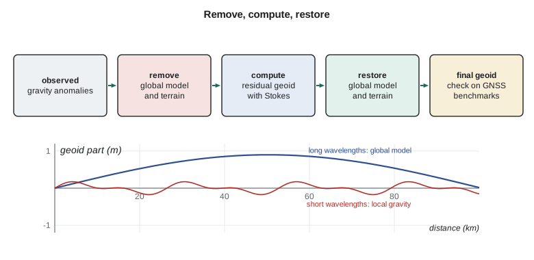
First, the long wavelengths are removed from the observed gravity anomalies using a global gravity model, typically one built from GRACE and GOCE for the long and medium wavelengths and terrestrial data for the rest. The effect of the topography is also removed, because masses above the geoid violate Stokes's assumption; this is done by computing their gravity from a digital elevation model and a density, often 2,670 kg/m³ for crustal rock. What remains is a set of small residual anomalies that vary smoothly enough to interpolate and that are dominated by local features.

Second, the residual geoid is computed from the residual anomalies with a modified form of Stokes's integral, over a cap of limited radius, often one or two degrees. The modification removes the long-wavelength part of the kernel so that the global model, not the sparse distant gravity, supplies those wavelengths. Several modifications are in use, named after the geodesists who proposed them, and choosing one is part of the art.

Third, the parts removed are restored: the global model's geoid and the indirect effect of the topography, which accounts for the shift between the geoid and the surface used in the computation after the masses were moved. Adding them gives the final geoid.

A small example

The code applies remove-compute-restore at one point in a toy area: a 5 by 5 grid of residual anomalies 10 km apart, with a local positive anomaly at the centre. It uses the planar approximation of Stokes's integral, which is adequate over a small area, and treats the central cell with a separate formula, as real software does, because the kernel is singular at the computation point. The global model part and the terrain restore are given numbers chosen for the CR1 area.

import math
# Remove-compute-restore on a small synthetic area (planar Stokes approximation).
# Residual gravity anomalies (mGal) on a 5 x 5 grid with 10 km spacing, after removing a global model.
dg = [[ 2.0,  4.0,  6.0,  3.0,  1.0],
      [ 3.0,  8.0, 12.0,  7.0,  2.0],
      [ 4.0, 11.0, 18.0, 10.0,  3.0],
      [ 2.0,  7.0, 11.0,  6.0,  1.0],
      [ 0.0,  2.0,  4.0,  2.0, -1.0]]
d = 10000.0                  # grid spacing, m
gamma = 9.806                # normal gravity, m/s2
# Planar Stokes kernel: N(P) = 1/(2 pi gamma) * sum( dg * dA / l ), inner zone handled with the circular-cell formula
def residual_geoid(i0, j0):
    s = 0.0
    for i in range(5):
        for j in range(5):
            g = dg[i][j] * 1e-5
            if (i, j) == (i0, j0):
                r0 = math.sqrt(d * d / math.pi)       # radius of a circle with the cell's area
                s += g * 2 * math.pi * r0 / (2 * math.pi)
            else:
                l = d * math.hypot(i - i0, j - j0)
                s += g * d * d / (2 * math.pi * l)
    return s / gamma
N_res = residual_geoid(2, 2)
N_glob = -16.375            # geoid height from the global model at the middle point, m
N_terr = -0.018            # indirect (terrain) effect restored, m
print(f"residual geoid from local gravity  {N_res * 100:+.2f} cm")
print(f"global model part                  {N_glob:+.3f} m")
print(f"terrain restore                    {N_terr * 100:+.2f} cm")
print(f"final geoid height                 {N_glob + N_res + N_terr:+.3f} m")
# Check against a benchmark with GNSS and a known height: N_obs = h - H
h, H = 893.412, 909.589
print(f"geoid from GNSS and benchmark      {h - H:+.3f} m")
print(f"difference (gravimetric - observed) {100 * (N_glob + N_res + N_terr - (h - H)):+.1f} cm")

residual geoid from local gravity  +23.58 cm
global model part                  -16.375 m
terrain restore                    -1.80 cm
final geoid height                 -16.157 m
geoid from GNSS and benchmark      -16.177 m
difference (gravimetric - observed) +2.0 cm

The residual anomalies, peaking at 18 mGal, contribute about +24 cm to the geoid at the centre. With the global model's −16.375 m and a terrain restore of −1.8 cm, the final geoid height is −16.157 m. The GNSS-levelling value at CR1 is −16.177 m, so the gravimetric model is 2.0 cm high there. A difference of a couple of centimetres is typical of a gravimetric geoid in the Prairies, and it is the reason agencies test models against GNSS on levelled benchmarks.

The toy example also shows how sensitive the result is to the nearest data. The central cell alone contributes a large share of the residual, and an error of a few milligals there would change the answer by a centimetre or more. Gravity coverage near the computation point, especially in rugged terrain, is what limits geoid accuracy on land.

Gravity data for geoid models

Three kinds of gravity data feed national geoid models. Terrestrial gravity, measured with relative gravimeters tied to absolute gravity stations, gives the most detail but is unevenly spread: dense along roads, sparse in mountains and forests. Marine gravity comes from ships and, offshore, from satellite altimetry, which maps the sea surface and so the marine geoid. Airborne gravity fills the gaps between land and sea and over rough terrain.

In Canada, the Canadian Geodetic Survey maintains the national gravity database, built over more than a century, and has used airborne surveys to fill gaps, notably in the mountains and the north. It also exchanges data with the United States, since the two countries' geoids must agree across the border.

Methods in practice

Stokes's integral is rarely evaluated point by point over a national grid, because a model has millions of nodes. Agencies use fast Fourier transform methods, which evaluate the convolution for the whole grid at once, or least-squares collocation, which treats the anomalies and geoid as correlated random fields and predicts the geoid with its error estimate. Collocation handles scattered data of different kinds naturally, including airborne gravity at flight height and deflections of the vertical, but is expensive for very large areas. Many national models use a combination: spectral methods for the main computation and collocation for gridding the data or for special regions.

There is also a choice of target surface. Stokes's approach computes the geoid, which lies inside the topography in mountains, so the density of the rock between the geoid and the surface must be assumed. Molodensky's approach, developed in the 1940s and 1950s, avoids that assumption by computing a surface close to the topography instead: the quasigeoid, which goes with normal heights rather than orthometric heights. The two differ by less than a centimetre in flat country but by decimetres in high mountains. Canada and the United States use the geoid and orthometric heights; much of Europe uses the quasigeoid and normal heights. Lesson 11 compares the height systems.

Finally, every gravity value must be consistent: in the same gravity datum, reduced with the same normal gravity formula, corrected for the same atmospheric effect, and referred to the same tide system. Merging data sets from different decades, instruments and agencies is often the largest single task in building a model. Errors such as a datum offset of a few milligals between two survey campaigns, or positions taken from old maps with errors of hundreds of metres, can each spoil a model locally, and finding them takes careful comparison with neighbouring data and with the satellite fields.

Gravimetric and hybrid models

A purely gravimetric geoid is computed from gravity alone. A hybrid geoid is a gravimetric geoid warped to fit the heights of benchmarks in an existing levelling-based datum, using GNSS on those benchmarks. Hybrid models give users heights consistent with the old datum; gravimetric models define the new datum itself.

In Canada, CGVD2013 is defined by a gravimetric geoid, so there is no hybrid step. Its current realization uses the model CGG2013a, and Natural Resources Canada has announced that the next realization will be based on SGEOID2022, a new gravimetric model computed jointly with the United States, while keeping the CGVD2013 name. A separate hybrid model, HTv2.0, lets users obtain heights in the old CGVD28 datum from GNSS.

Testing a geoid model

Agencies test geoid models in three main ways. GNSS on levelled benchmarks compares N from the model with h − H, as in the code; the differences show both the geoid's errors and the levelling network's, so a long-wavelength tilt may belong to either. Astrogeodetic deflections of the vertical, measured with modern digital zenith cameras, test the geoid's slope. And dedicated geoid slope validation surveys, of which NGS ran three in the 2010s along lines in Texas, Iowa and Colorado, measure the geoid along a profile with GNSS, levelling, gravity and deflections so precisely that models can be judged to a centimetre over hundreds of kilometres.

The best modern models reach about 1 to 2 cm in flat, well-surveyed regions and several centimetres in mountains. The international target for a geoid-based height datum is about a centimetre, consistent with what GNSS can deliver in ellipsoidal height on a long session.

The geoid changes with time

A geoid computed from gravity is a snapshot. Where the mass of the Earth changes, the geoid changes with it. Glacial isostatic adjustment raises the geoid slowly over Hudson Bay, by roughly a millimetre per year at the centre of uplift; melting glaciers lower it nearby; and large water storage changes affect it seasonally by a few millimetres. For a datum meant to last decades, these changes are modelled, and the new North American vertical datums include, or will include, a model of the geoid's change with time.

Coulee Geomatics: a local geoid check

The district's engineers want heights at the new pump station and along the canal that agree with the levelled benchmarks to a centimetre, from GNSS alone. Leah sets up a test before trusting any model. Grant and Ines occupy six benchmarks spread over the district for four hours each with GNSS, and Theo computes h − H at each and compares it with the national model. If the misfits are a few centimetres and nearly constant, a simple fitted offset is enough for the project; if they show a tilt or a local bump, the model or the levelling has a problem worth reporting to the agency. In this case the misfits average +1.9 cm with a spread of 0.8 cm, so the firm adopts the national model with a documented offset for the project, and sends the results to the agency, which collects such comparisons to improve future models.

Ruth adds one rule to the project's specifications: any height derived from GNSS must state the geoid model, the datum, the epoch and the offset applied. A height without those four labels cannot be checked later, and the change of vertical datum in lesson 11 would make it ambiguous.