
GEOM-430 · Lesson 5 of 12 · 21 min
Satellite gravimetry
GEOM-230 introduced the gravity field as the reason heights and the geoid exist. Measuring that field used to mean carrying gravimeters across the land and towing them behind ships, a slow and uneven business that left large parts of the world unsurveyed. Since 2000, a series of satellite missions has mapped the global field from orbit, and two of them have done something no ground survey could: they have measured how the field changes from month to month as water, ice and air move around the planet. This lesson explains how satellites sense gravity, how the results are expressed, and what they have revealed.
Gravity from orbit
A satellite in free fall follows the gravity field, so its orbit carries information about the field. The trouble is that the field's fine detail fades rapidly with height. At altitude r, the part of the potential described by spherical harmonics of degree n is reduced by a factor of about (R/r) to the power n+1 compared with its value at the surface. A satellite 400 km up sees the long-wavelength shape of the field clearly but the shorter wavelengths only faintly. Satellite gravimetry is therefore a contest between flying low, to see more detail, and staying up long enough to be useful, since atmospheric drag pulls low satellites down.
The coefficients C and S of this expansion are what gravity missions estimate. Degree n corresponds to a half-wavelength of about 20,000/n km at the surface, so a model complete to degree 200 resolves features about 100 km across, and degree 2160, as in the global models used for geoid work, about 9 km. The degree-2 zonal coefficient, related to J₂, describes the Earth's flattening and is by far the largest after the central term.
The missions
| Mission | Years | Principle | Main result |
|---|---|---|---|
| CHAMP | 2000 to 2010 | GPS tracking of a single low satellite | First consistent global field from one mission |
| GRACE | 2002 to 2017 | Microwave ranging between two satellites about 220 km apart | Monthly fields showing mass change |
| GOCE | 2009 to 2013 | Gradiometer measuring gravity differences inside the satellite, very low orbit | Static field to about 100 km resolution |
| GRACE-FO | 2018 onward | As GRACE, plus a laser ranging interferometer | Continuation of the monthly record |
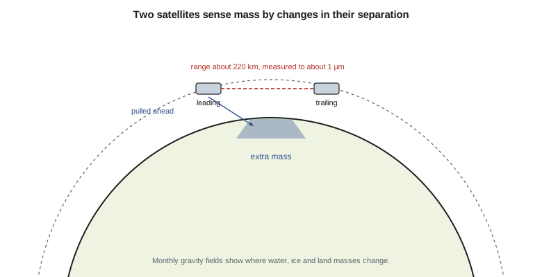
GRACE, the Gravity Recovery and Climate Experiment, was a joint mission of NASA and the German Aerospace Center. Two identical satellites flew one behind the other in the same orbit, linked by a microwave system that measured the changing distance between them to a few micrometres. When the leading satellite approaches a region of extra mass, it is pulled ahead and the gap widens; the trailing satellite is then pulled ahead in turn and the gap closes. GPS receivers tracked both satellites, accelerometers measured the non-gravitational forces such as drag, and from all of this a new gravity field was computed every month.
GRACE Follow-On, launched in 2018, continues the record after a gap of about a year. It also carries a laser ranging interferometer, a technology demonstration that measured the separation far more precisely than the microwave system. The next mission, GRACE-C, led by NASA and the German Aerospace Center, will use the laser instrument as its main ranging system and is planned for launch in about 2028, overlapping with GRACE-FO. Europe and the United States are also studying pairs of such missions in different orbits, which would see changes in more detail and more often.
GOCE, the Gravity field and steady-state Ocean Circulation Explorer of the European Space Agency, took a different approach. It carried a gradiometer: six accelerometers in a rigid frame measuring differences in gravity over half a metre inside the spacecraft. To sense fine detail it flew remarkably low, about 255 km and later lower, with an electric ion engine to cancel the drag. Its static field, combined with GRACE for the longest wavelengths and with ground data for the shortest, underpins most modern geoid models, including those in Canada and the United States.
Time-variable gravity and mass change
The most surprising discovery of GRACE was how much the gravity field changes. A monthly field differs from the long-term average mainly because water moves: snow accumulates and melts, soil moisture and groundwater rise and fall, lakes and reservoirs fill, ice sheets lose mass, and the ocean's mass redistributes. Over a region, the change in the field can be converted into the change in surface mass, usually expressed as equivalent water height: the thickness of a layer of water that would cause the same change.
Here ρₑ is the mean density of the Earth and kₙ are load Love numbers, which account for the solid Earth's elastic response to the load. In practice the coefficients are noisy at high degrees and show stripes along the satellite tracks, so they are filtered, and many users prefer mascon solutions: fields estimated directly as mass changes in a grid of blocks a few hundred kilometres across, with constraints that reduce the noise. The NASA Jet Propulsion Laboratory, the University of Texas Center for Space Research and the German Research Centre for Geosciences publish such products monthly.
import math
GM = 3.986004418e14; a = 6378137.0
# 1. The effect of the Earth's flattening term J2 on gravity at the pole and equator (spherical approximation)
J2 = 1.08263e-3
for name, lat in (("equator", 0.0), ("45 deg", 45.0), ("pole", 90.0)):
    s = math.sin(math.radians(lat))
    P2 = 0.5 * (3 * s * s - 1)
    g0 = GM / a ** 2
    dg = g0 * 3 * J2 * P2          # radial derivative of the degree-2 term at r = a
    print(f"{name:8s} J2 changes attraction by {dg * 1e5:+9.1f} mGal")
# 2. Converting a GRACE trend in equivalent water height to mass
area_km2 = 400000           # area of the region, km2
ewh_cm_per_yr = -1.2       # trend, cm of water per year (illustrative)
mass_gt = area_km2 * 1e6 * ewh_cm_per_yr / 100 * 1000 / 1e12
print(f"region {area_km2:,} km2, trend {ewh_cm_per_yr:+.1f} cm/yr of water")
print(f"mass change {mass_gt:+.1f} Gt per year")
print(f"sea level equivalent {-mass_gt / 362:+.3f} mm per year")
# 3. The resolution rule: degree n resolves features of about half-wavelength 20000/n km
for n in (60, 90, 200):
    print(f"degree {n:3d}: half-wavelength about {20000 / n:.0f} km")
# 4. Gravity change from a 1 m layer of water spread over a large area (Bouguer plate)
G = 6.674e-11
print(f"1 m of water as an infinite slab: {2 * math.pi * G * 1000 * 1 * 1e8:.1f} microGal")equator J2 changes attraction by -1591.2 mGal 45 deg J2 changes attraction by +795.6 mGal pole J2 changes attraction by +3182.4 mGal region 400,000 km2, trend -1.2 cm/yr of water mass change -4.8 Gt per year sea level equivalent +0.013 mm per year degree 60: half-wavelength about 333 km degree 90: half-wavelength about 222 km degree 200: half-wavelength about 100 km 1 m of water as an infinite slab: 41.9 microGal
The first part shows why J₂ dominates: in this spherical approximation the flattening term changes the attraction by about 1,600 mGal at the equator and 3,200 mGal at the poles, of the same order as the full difference in normal gravity between pole and equator in GEOM-230, about 5,200 mGal, the rest of which comes from rotation. The second part converts an illustrative drought trend over the southern Prairie region, −1.2 cm of water per year over 400,000 km², into about −4.8 Gt per year. That is a large amount of water for the region's farms and rivers, but it would raise global sea level by only about 0.01 mm per year if it all reached the ocean. The last line shows that a 1 m layer of water spread widely changes gravity by about 42 microgal, which a modern absolute gravimeter can detect.
What GRACE has shown
Two decades of monthly fields have changed hydrology and climate science. They show the Greenland and Antarctic ice sheets losing hundreds of gigatonnes of ice per year, with large year-to-year swings tied to weather. They show the depletion of major aquifers where irrigation pumps groundwater faster than it recharges, including in the southern High Plains of the United States, northern India and the Middle East. They show the seasonal swelling and draining of the great river basins, the filling of reservoirs, and the effects of droughts and floods. Lesson 12 returns to the ice sheets and sea level.
In Canada, GRACE fields have been used to study the water balance of the Prairies and the Mackenzie and Nelson river basins, and to separate glacial isostatic adjustment, which shows up as a slow increase in mass around Hudson Bay as mantle rock flows back under the rising crust, from changes in water storage. That separation needs both GRACE and GNSS: GNSS measures the uplift, GRACE the mass change, and models of the Earth's interior relate the two.
Gravity on the ground
Satellite fields are calibrated and extended by measurements on the ground. Absolute gravimeters drop a corner-cube reflector in a vacuum chamber and track its fall with a laser interferometer, timing it against an atomic clock, to measure gravity to a few microgal: a few parts in a billion of the total. Relative gravimeters, which measure differences from a reference station with a spring or a superconducting sphere, are faster and cheaper but drift and must be tied to absolute stations. Superconducting gravimeters at a handful of observatories record gravity continuously for years, detecting the tides, the loading of the atmosphere and groundwater, and the slow change due to GIA.
Repeated absolute gravity measurements at the same site, combined with GNSS heights, give a direct test of models of glacial isostatic adjustment: if the ground rises because rock flows back underneath, gravity decreases by about 0.15 to 0.2 microgal for each millimetre of uplift, which is less than the free-air rate of 0.3 microgal per millimetre because mass is added. Long series of such measurements have been made at sites in central Canada and the northern United States for exactly this purpose.
Limits of satellite gravimetry
Satellite gravity fields are smooth by nature. GRACE resolves changes over areas of about 300 km and larger, and a signal in one place leaks into its neighbours when the field is filtered, so a small catchment or a single reservoir cannot be studied directly. The monthly fields also have errors that grow towards higher degrees, and the lowest-degree terms, especially the change in C₂₀ and the position of the centre of mass (degree 1), are poorly determined by GRACE itself and are taken from SLR. That is another example of the techniques supporting each other.
For static geoid work, the satellites provide the long and medium wavelengths, to a few hundred kilometres for GRACE and about 100 km for GOCE. The shorter wavelengths, which matter most for heights in hilly country, still come from terrestrial, airborne and marine gravity and from terrain models. Lesson 6 shows how these pieces are combined.
Worked problem
Mass and sea level equivalent
An ice cap loses 50 Gt of ice per year. How much does that raise global mean sea level?
Show solution
- \[\Delta h = \frac{50}{362} = 0.138\ \text{mm/yr}\]
Answer: About 0.14 mm per year, using 362 Gt of water per millimetre of global sea level.
Coulee Geomatics and the reservoir
The university research group wants to know whether the diversion dam's reservoir, which rises several metres each spring, measurably loads the crust. Its area is far too small for GRACE, which would see only the regional water balance. But the load is close to CR1 and the monitoring pillars, and the vertical response of the ground can be computed from the reservoir's level using elastic loading theory, the same theory behind the load Love numbers. Leah sets up the comparison: CR1's daily vertical positions against the reservoir level, with the regional GRACE signal removed. The expected effect is a fraction of a millimetre, so the result will depend on a long, clean record, and on removing every other vertical signal first: the atmosphere's load, the seasonal soil moisture cycle and the slow GIA trend. If the effect can be seen at all, it will be the first measurement of the reservoir's load on the crust in the district.
Common mistakes
MistakeExpecting GRACE to resolve a single reservoir or small watershed.
InsteadIts resolution is about 300 km; use it for regional mass change.
MistakeTreating a monthly gravity field as noise-free.
InsteadFilter the coefficients or use mascon solutions, and account for leakage.
MistakeUsing GRACE alone for the lowest-degree terms.
InsteadTake C₂₀ and degree 1 from SLR and other sources.
MistakeAssuming satellites have replaced ground gravity for geoid work.
InsteadShort wavelengths still need terrestrial, airborne and terrain data.
Summary and key terms
- Satellite orbits sense the gravity field, but fine detail fades with height.
- Fields are expressed as spherical harmonic coefficients; degree n resolves about 20,000/n km.
- GRACE and GRACE-FO measure the field monthly from the changing distance between two satellites.
- GOCE's gradiometer mapped the static field to about 100 km.
- Changes in gravity are converted to equivalent water height and mass.
- GRACE has measured ice sheet loss, aquifer depletion and seasonal water storage.
- Spherical harmonics
- Functions on a sphere used to express the gravity field by degree and order.
- Equivalent water height
- The thickness of a water layer that would cause an observed mass change.
- Mascon
- A mass concentration block used to estimate mass change directly.
- Gradiometer
- An instrument measuring differences in gravity over a short baseline.
- Load Love number
- A number describing the elastic deformation of the Earth under a surface load.
- GRACE-FO
- The follow-on to GRACE, launched in 2018 and carrying a laser ranging interferometer.
Practice problems
Work each problem on paper first, then reveal the answer to check.
Which degree of spherical harmonic resolves features about 200 km across (half-wavelength)?
Show answer
About degree 100.
How do GRACE satellites sense extra mass beneath them?
Show answer
The leading satellite is pulled ahead, changing their separation.
Convert 362 Gt of water to global sea level.
Show answer
About 1 mm.
Why did GOCE fly so low?
Show answer
To sense shorter wavelengths of the field, which fade with height.
Which lowest-degree terms are taken from SLR for GRACE solutions?
Show answer
C₂₀ and the degree-1 terms (the centre of mass).
Lesson quiz · 5 questions
Score 60% or more to complete this lesson.
Create a free account to save your progress, take quizzes and earn a certificate.