
GCP-221 · Lesson 4 of 12 · 19 min
Partitioning, clustering and query cost
▶ Video coming soon A video version of this lesson is on the way.
Friday, October 16, is cost day. Ravi opens the job history query from lesson 1 and points to the dashboard tile that scanned the whole web events table each time anyone opened the marketing report: about 1,400 GiB per view. In September the report was opened 212 times. Mateo works out the bill on the spot. At 6.25 US dollars per TiB, each view cost about 8.54 US dollars, and the month cost a little over 1,800 US dollars for one tile that showed yesterday's visits. The fix takes ten minutes, and it uses the two features this lesson covers.
Partitioned tables
A partitioned table is divided into segments, called partitions, based on the value of one column. Queries that filter on that column read only the matching partitions, a behaviour called partition pruning. BigQuery supports three kinds of partitioning.
| Type | Partition column | Example | Notes |
|---|---|---|---|
| Time-unit column | A DATE, TIMESTAMP or DATETIME column | curated.sales by sale_date, daily | Hourly, daily, monthly or yearly partitions |
| Ingestion time | The time BigQuery received the row (_PARTITIONTIME) | A raw landing table | Useful when the data has no reliable date of its own |
| Integer range | An INT64 column split into ranges | Customers by customer_id in ranges of 100,000 | Less common for analytics |
Birchline's curated tables are partitioned by their business date: sales by sale_date and web events by event_date, one partition per day. A table can have up to 10,000 partitions, which is more than 27 years of daily partitions. Two table options make partitioning safer. Require partition filter makes BigQuery reject any query on the table that does not filter on the partition column, which stops accidental full scans. Partition expiration deletes partitions older than a set number of days automatically, which suits raw and scratch data.
Pruning only works when the filter can be worked out before the query runs. A filter such as WHERE event_date = "2026-10-15" or WHERE event_date >= DATE_SUB(CURRENT_DATE(), INTERVAL 7 DAY) prunes. A filter that depends on another table, such as WHERE event_date IN (SELECT ...), or a filter that wraps the column in a function that changes its type, may not prune, and the dry run will show the full table size. The rule of thumb is to compare the partition column directly with a constant or a simple date expression.
Clustered tables
Clustering sorts the data within each partition by up to four columns. BigQuery stores the sorted data in blocks and keeps the minimum and maximum values of the clustering columns for each block. When a query filters on a clustering column, BigQuery skips blocks whose range cannot contain the value. Clustering also helps queries that aggregate or join on the clustering columns.
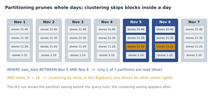
Curated sales is clustered by store_id and then sku, because most reports filter or group by store, and product-level analysis filters by SKU. The order of clustering columns matters: blocks are sorted by the first column, then the second within it, so a filter on sku alone helps less than a filter on store_id. Clustering works best on columns with many distinct values that queries filter on often.
One difference between the two features shows up in cost estimates. Partition pruning is known before the query runs, so the dry run's estimate already reflects it. The benefit of clustering is only known while the query runs, so the estimate shows the size after pruning partitions, and the bytes actually billed are lower. Analysts sometimes think clustering is not working because the estimate does not change; the job details after the run tell the real story.
| Feature | Partitioning | Clustering |
|---|---|---|
| Columns | One | Up to four, in order |
| Cost known in advance | Yes, the dry run shows pruning | No, savings appear after the run |
| Best for | Filters on a date or range; expiring old data | Filters and grouping on high-cardinality columns |
| Limits | Up to 10,000 partitions | No partition count limit; automatic re-clustering |
| Use together? | Yes: partition by date, cluster by the columns filtered next | Yes |
Fixing the marketing tile
The marketing tile's query counted yesterday's visits by device, but its filter was written as WHERE DATE(event_ts) = DATE_SUB(CURRENT_DATE(), INTERVAL 1 DAY). Because it filtered on event_ts converted to a date, not on the partition column event_date, BigQuery could not prune, and every view read every partition. Changing one line fixed it.
-- Before: no pruning, about 1,400 GiB per run
SELECT device, COUNT(DISTINCT session_id) AS sessions
FROM `bl-data-prod.curated.web_events`
WHERE DATE(event_ts) = DATE_SUB(CURRENT_DATE(), INTERVAL 1 DAY)
GROUP BY device;

-- After: filters the partition column, about 0.3 GiB per run
SELECT device, COUNT(DISTINCT session_id) AS sessions
FROM `bl-data-prod.curated.web_events`
WHERE event_date = DATE_SUB(CURRENT_DATE("America/Toronto"), INTERVAL 1 DAY)
GROUP BY device;
The new filter also gives CURRENT_DATE a time zone. Without it, CURRENT_DATE uses UTC, and in the evening in Toronto "yesterday" in UTC is already the local today. Ravi also sets require partition filter on curated.web_events, so the old pattern can never come back.
On-demand and capacity pricing
Under on-demand pricing, each project pays for the bytes its queries scan, at 6.25 US dollars per TiB in the US multi-region at the time of writing, and the first TiB each month is free. Each query is billed at least 10 MB for each table it references. On-demand is simple and suits teams whose usage is moderate or unpredictable.
Under capacity pricing, the organization buys slot capacity through a BigQuery edition: Standard, Enterprise or Enterprise Plus. Capacity is measured in slots and billed per slot-hour, with autoscaling that adds slots when queries need them, and optional one-year or three-year commitments for a lower rate. The published pay-as-you-go rates in the US are about 0.04 US dollars per slot-hour for Standard, 0.06 for Enterprise and 0.10 for Enterprise Plus. Higher editions add features such as more security controls and longer retention options. A reservation assigns capacity to projects, so different teams can have guaranteed slots.
| Question | On-demand | Capacity (editions) |
|---|---|---|
| What you pay for | Bytes scanned by each query | Slot-hours, used or committed |
| Cost predictability | Varies with what people query | Predictable with commitments and limits on autoscaling |
| Best fit | Moderate or irregular use; small teams | Heavy, steady use; many dashboards and pipelines |
| Effect of a careless SELECT * | A direct, possibly large bill | Uses slots and slows others, but no extra charge per byte |
| Cost controls | Maximum bytes billed, custom quotas per user or project | Reservation size, autoscaling maximum, assignments |
Ravi asks Mateo to compare the two for the analytics project using last month's figures: 38 TiB scanned in total, mostly by dashboards during business hours, not counting the marketing tile. The calculation below uses the published rates and an illustrative capacity pattern.
tib_scanned = 38          # last month, analytics project
free_tib = 1
on_demand_rate = 6.25     # US dollars per TiB
on_demand = (tib_scanned - free_tib) * on_demand_rate

# Illustrative capacity plan: Enterprise edition, autoscaling
rate = 0.06               # US dollars per slot-hour, pay as you go
baseline_slots = 50       # always on
busy_extra_slots = 100    # autoscaled during business hours
busy_hours = 10 * 22      # 10 hours a day, 22 working days
hours_in_month = 24 * 30
capacity = baseline_slots * hours_in_month * rate + busy_extra_slots * busy_hours * rate

print(f"On-demand: {on_demand:,.2f} US dollars")
print(f"Capacity:  {capacity:,.2f} US dollars")
print(f"Break-even TiB scanned: {capacity / on_demand_rate + free_tib:.1f}")On-demand: 231.25 US dollars Capacity: 3,480.00 US dollars Break-even TiB scanned: 557.8
What this code does
Comparing a month of on-demand billing with an illustrative capacity plan. The on-demand cost is the TiB scanned, less the free TiB, times the price per TiB. The capacity cost is the always-on slots for every hour of the month plus the extra slots during business hours, times the price per slot-hour. The output shows that at this level of use on-demand is cheaper, and how many TiB a month the team would have to scan before capacity pricing paid for itself.
At 38 TiB a month, on-demand costs 231.25 US dollars and the illustrative capacity plan costs 3,480 US dollars, so on-demand is the clear choice for now. The break-even point is around 558 TiB a month. The exercise also shows why cost management on on-demand is about bytes: the 1,800-dollar tile was almost eight times the rest of the month's bill.
Other ways to reduce cost and time
Partitioning and clustering do the most, but several other habits help. Select only the columns you need. Filter early, in the first CTE, rather than after joins. Use approximate functions for large distinct counts when an estimate is acceptable. Preview tables instead of querying them. Materialize results that many people read, which lesson 5 covers. Set maximum bytes billed on scheduled queries and custom quotas that cap how much a user or project can scan per day. And remember that BI Engine, an in-memory accelerator, can make dashboard queries much faster; with editions, a reservation includes some BI Engine capacity, and on-demand projects can buy it separately.
Storage cost matters less than query cost for most analytics teams, but it is not zero. Active logical storage in the US costs about 0.023 US dollars per GiB per month, and data that has not changed for 90 days drops to the long-term rate of about 0.016. Long-term pricing applies automatically to each partition separately, so in a daily partitioned table, old days become cheaper without anyone doing anything, as long as nobody rewrites them.
Common mistakes
MistakeFiltering on a function of a timestamp instead of the partition column.
InsteadFilter the partition column directly, such as event_date = a date, so BigQuery can prune.
MistakeExpecting the dry run to show clustering savings.
InsteadThe estimate reflects partition pruning only; check bytes billed after the run for clustering.
MistakeChoosing capacity pricing for a small team because it sounds more professional.
InsteadCompare real usage: below the break-even point, on-demand is cheaper.
MistakeClustering on a column queries rarely filter on.
InsteadCluster on the columns used in filters and grouping, most important first.
Watching cost over time
Fixing one expensive tile is useful; noticing the next one early is better. Ravi sets up three simple habits for the team. First, a weekly query on INFORMATION_SCHEMA.JOBS lists the ten queries with the most bytes billed, grouped by the query's text with dates removed, so that a dashboard tile that runs hundreds of times shows up as one line with its total. Second, Cloud Billing budgets and alerts on the analytics project send an email to the team when monthly spending passes half, three quarters and all of the planned amount. Third, the custom quota on the project caps how many bytes each user can scan per day, set high enough for normal work but low enough that a runaway query stops long before it becomes a large bill.
Mateo asks whether the team should simply move to capacity pricing to make costs predictable. Ravi's answer is that predictability has a price: on the numbers from this lesson, the team would pay many times more for slots it does not need. The better path is to keep on-demand pricing, make queries efficient, and revisit the decision each quarter with real usage, because the break-even point moves as dashboards and pipelines grow. Choosing a pricing model is not a one-time decision; it is a measurement repeated as the workload changes.
Worked problem
The cost of one dashboard tile
A tile scanned 1,400 GiB per view and was opened 212 times in a month. After the fix it scans 0.3 GiB per view. At 6.25 US dollars per TiB, what did the month cost before and after?
Show solution
- Before, per view: 1,400 / 1,024 = 1.367 TiB, times 6.25 = 8.54 US dollars.
- Before, per month: 8.54 x 212 = 1,811 US dollars, about 1,810.
- After, per view: 0.3 / 1,024 = 0.000293 TiB, times 6.25 = 0.0018 US dollars.
- After, per month: 0.0018 x 212 = 0.39 US dollars.
Answer: About 1,810 US dollars before and under 40 cents after, for exactly the same chart.
Summary and key terms
- Partitioning divides a table by a date, ingestion time or integer range so queries read only the partitions they filter on.
- Pruning needs a direct filter on the partition column; require partition filter blocks full scans, and partition expiration deletes old data.
- Clustering sorts data within partitions by up to four columns and lets BigQuery skip blocks, with savings that show only after the query runs.
- On-demand pricing bills bytes scanned at 6.25 US dollars per TiB with a free TiB each month; capacity pricing bills slot-hours through Standard, Enterprise or Enterprise Plus editions.
- Compare real usage to choose.
- Maximum bytes billed, quotas, materialized results and BI Engine help control cost.
- Unchanged partitions move to cheaper long-term storage after 90 days.
- Partitioned table
- A table divided into segments by the value of one column.
- Partition pruning
- Skipping partitions that a query's filter excludes.
- Require partition filter
- A table option that rejects queries without a filter on the partition column.
- Clustering
- Sorting data within partitions by up to four columns so blocks can be skipped.
- BigQuery editions
- Standard, Enterprise and Enterprise Plus capacity offerings billed by slot-hour.
- Reservation
- An allocation of slot capacity assigned to projects.
- Maximum bytes billed
- A limit that makes a query fail rather than scan more than a set amount.
- BI Engine
- An in-memory accelerator for dashboard queries.
Practice problems
Work each problem on paper first, then reveal the answer to check.
Why did WHERE DATE(event_ts) = ... read the whole table?
Show answer
It filtered on a function of event_ts, not on the partition column event_date, so BigQuery could not prune.
Why does the dry run not show savings from clustering?
Show answer
Clustering benefits are only known while the query runs; the estimate reflects partition pruning only.
When does capacity pricing make sense?
Show answer
When steady, heavy use costs more on demand than the slot capacity needed, past the break-even point.
What happens to the storage price of a partition that has not changed for 90 days?
Show answer
It drops to the long-term rate automatically.
Lesson quiz · 5 questions
Score 60% or more to complete this lesson.
Create a free account to save your progress, take quizzes and earn a certificate.