
GCP-221 · Lesson 1 of 12 · 20 min
BigQuery architecture for analysts
▶ Video coming soon A video version of this lesson is on the way.
On Wednesday, October 7, the day after his first data preparation session, Mateo Alvarez sits down with Ravi Menon for the first of a second set of sessions. The Tuesday and Thursday sessions cover getting data into Birchline's warehouse cleanly. These Wednesday and Friday sessions cover the other half of an analyst's job: asking questions of that data, turning the answers into reports and dashboards, and explaining what they mean. Ravi has one goal for the series. By the middle of November, Mateo should be able to take a question from Lena Okafor, Birchline's director of retail operations, and return a correct, well-explained dashboard that store managers can trust.
Mateo is not new to analysis. For two years he built sales reports for the stores team from spreadsheets and a few saved BigQuery queries that someone else had written. What he has never had is a clear picture of how BigQuery works underneath. Ravi starts there, because almost every decision an analyst makes about speed and cost follows from the architecture.
What BigQuery is
BigQuery is Google Cloud's serverless data warehouse. "Serverless" means there are no machines for the analyst to size, start or patch. You create datasets and tables, load or stream data into them, and run SQL. Google runs the hardware, spreads the work across many machines and bills for what you store and what you process. For an analyst, that means the first questions are not "how big a server do we need?" but "how much data will this query read?" and "who should be able to see this table?"
BigQuery organizes data in a simple hierarchy. A project is the unit of billing and access, such as bl-data-prod. A dataset is a container of tables in one location, such as curated or reference. A table holds rows with a schema. Views, materialized views, models and routines also live inside datasets. A table is always referred to in full as project.dataset.table, for example bl-data-prod.curated.sales, and many errors in shared queries come from leaving out the project and accidentally querying a table of the same name in a different project.
| Object | Example at Birchline | What it controls |
|---|---|---|
| Project | bl-data-prod | Billing, quotas, the top level of access |
| Dataset | curated | Location (region or multi-region), default expiration, dataset-level access |
| Table | curated.sales | Schema, partitioning, clustering, table-level access |
| View | curated.v_store_daily | A saved query that others can query like a table |
| Model | analytics.return_risk | A BigQuery ML model trained with SQL |
Storage and compute are separate
The single most useful idea in BigQuery is that storage and compute are separate. Data is stored in Google's distributed file system, Colossus, in a compressed columnar format. Queries are run by a separate engine, known internally as Dremel, which borrows units of processing called slots from a large shared pool, reads the columns it needs over Google's fast internal network, and returns the result. Storage and compute scale independently: a table can grow to many terabytes without any change to how queries run, and a busy morning of dashboards can use more slots without anyone adding disks.
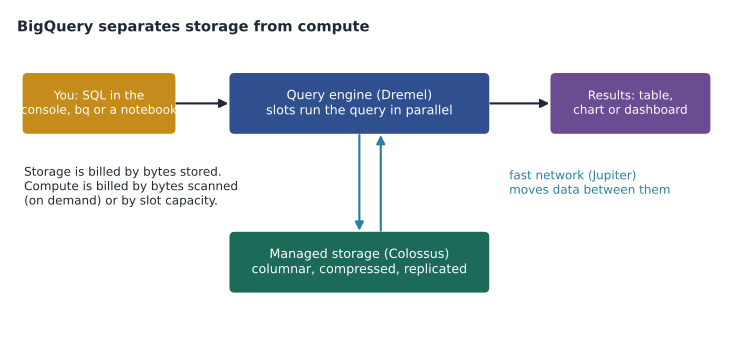
This separation explains BigQuery's two kinds of charge. Storage is billed for the bytes kept in tables, with a lower rate for data that has not been changed for 90 days. Compute is billed in one of two ways. Under on-demand pricing, each query is charged for the bytes it scans. Under capacity pricing, through BigQuery editions, the organization pays for slot capacity over time and queries are not charged by bytes. Lesson 4 works through both. For now, the key point is that under on-demand pricing, which Birchline's analytics project uses, the cost of a query depends on how much data it reads, not on how long it runs or how complicated the SQL looks.
Columnar storage: why SELECT star is expensive
A traditional transactional database stores each row together: all the values for one sale sit next to each other on disk. That is ideal for an application that reads or writes one sale at a time. Analytical queries are different. They usually read a few columns from millions of rows, such as the store, the date and the sales amount, and add them up. BigQuery stores each column separately, so a query that names three columns reads only those three columns.
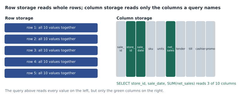
Two practical rules follow. First, **SELECT * is the most expensive way to look at a table**, because it reads every column. To preview data, use the table's Preview tab in the console, which is free, or select only the columns you need. Second, LIMIT does not reduce the bytes scanned for an ordinary table. A query with LIMIT 10 still reads every row of the columns it names, because the limit is applied after the scan. Mateo admits that his habit of typing SELECT * ... LIMIT 10 to look at a new table has been costing money every time.
Columnar storage also compresses well. Values in one column are similar: the store_id column holds the same forty values over and over, and a column of booleans is almost all false. BigQuery stores these columns in a compressed form, so the stored size is often much smaller than the raw file that was loaded. Billing for scans, however, is based on the logical size of the data, which is the uncompressed size of each data type. An INT64 counts as 8 bytes and a STRING as 2 bytes plus its length in UTF-8, whatever the compression.
Estimating a query before running it
Because cost follows bytes scanned, BigQuery shows the estimate before you run anything. In the console, the query validator in the top right of the editor shows a message such as "This query will process 2.31 GB when run" as soon as the SQL is valid. From the command line, the same estimate comes from a dry run, which checks the query and reports the bytes without running it or charging for it.
bq query --use_legacy_sql=false --dry_run '
SELECT store_id, sale_date, SUM(net_sales) AS net_sales
FROM `bl-data-prod.curated.sales`
WHERE sale_date BETWEEN "2026-10-01" AND "2026-10-06"
GROUP BY store_id, sale_date'

# Query successfully validated. Assuming the tables are not modified,
# running this query will process 9437184 bytes of data.
The estimate is an upper bound for on-demand billing. If a table is clustered, the actual bytes can be lower, because BigQuery may skip blocks while it runs. The estimate is also why Ravi asks everyone to read the validator message before pressing Run on any unfamiliar table, and why the analytics project has a maximum bytes billed setting on scheduled queries: a query that would scan more than the limit fails instead of running up a bill.
To make the cost of column choice concrete, Ravi asks Mateo to estimate a query against the web events table, which holds about 1,400 GiB of clickstream data in 25 columns. The Python below uses the logical sizes of the columns Mateo might select and turns bytes into an on-demand cost at the published US rate of 6.25 US dollars per TiB.
# Logical size of each column of curated.web_events, in GiB (illustrative)
columns = {
    "event_ts": 89, "event_date": 45, "session_id": 160, "user_pseudo_id": 150,
    "event_name": 70, "page": 210, "product_sku": 60, "device": 40, "region": 35,
}
other_columns_gib = 1400 - sum(columns.values())   # the remaining 16 columns
price_per_tib = 6.25                               # US multi-region, on demand

def cost(gib):
    return gib / 1024 * price_per_tib

star = 1400
picked = columns["event_date"] + columns["event_name"] + columns["device"]
print(f"SELECT * reads {star} GiB, about {cost(star):.2f} US dollars")
print(f"3 columns read {picked} GiB, about {cost(picked):.2f} US dollars")
print(f"Share of bytes avoided: {1 - picked / star:.3f}")
print(f"Other 16 columns hold {other_columns_gib} GiB")SELECT * reads 1400 GiB, about 8.54 US dollars 3 columns read 155 GiB, about 0.95 US dollars Share of bytes avoided: 0.889 Other 16 columns hold 541 GiB
What this code does
Comparing what SELECT * costs on the web events table with a query that names three columns. Each column has a size in gibibytes, and the cost function turns gibibytes into tebibytes and multiplies by the on-demand price. The output shows that reading everything costs a little over eight dollars while three columns cost under a dollar, and that close to nine tenths of the bytes are avoided by naming columns.
The comparison does not yet use the date. Lesson 4 adds partitioning, which lets a query that filters on event_date skip whole days of data, and the savings multiply.
Where analysts write and run queries
BigQuery offers several places to work, and the Associate Data Practitioner exam expects you to know what each is for.
| Tool | Best for | Notes |
|---|---|---|
| BigQuery Studio (the console) | Writing and running SQL, previewing tables, saving queries | Query validator shows bytes; results can go to a chart, Sheets or Data Studio |
| Colab Enterprise notebooks in BigQuery | Mixing SQL, Python and charts for exploration | Managed Jupyter notebooks; can use BigQuery DataFrames |
| bq command-line tool | Scripts, dry runs, loading and exporting | Part of the Google Cloud CLI |
| Data canvas | Exploring visually with natural language and a graph of steps | Uses Gemini in BigQuery; lesson 7 |
| Connected Sheets | Business users who live in Google Sheets | Pivot and chart billions of rows from Sheets; lesson 10 |
| Data Studio and Looker | Reports, dashboards and governed models | Lessons 8 and 9 |
Notebooks deserve a word, because the exam names them explicitly. Colab Enterprise notebooks run inside BigQuery Studio, so an analyst can write a SQL cell, pull the result into Python, compute something that is awkward in SQL and draw a chart, all in one document that can be shared with colleagues. For large data, the BigQuery DataFrames library lets Python code that looks like pandas run inside BigQuery rather than on the notebook's own machine. Ravi's rule is simple: if the answer is a table or a number, write SQL; if the work is exploratory and mixes steps, use a notebook; if other people will look at it every week, build a report.
Locations, caching and other things that surprise new analysts
Each dataset lives in one location. Birchline keeps its analytics data in the northamerica-northeast2 (Toronto) region, and a query cannot join tables from datasets in different locations. When an exam question describes a query that fails because two tables are in different places, the fix is to copy one dataset to the other's location, not to change the SQL.
BigQuery caches query results for about 24 hours. If the same user runs exactly the same query again and the underlying tables have not changed, the result comes from the cache, quickly and at no charge. The cache does not help when the query text differs even slightly, when the tables have changed, or when the query uses functions such as CURRENT_TIMESTAMP whose results change. Dashboards benefit from caching, which is one reason a well-built report can be cheaper than a set of people each running their own slightly different queries.
Finally, jobs are the record of everything BigQuery runs. Each query, load or export is a job with an ID, a user, bytes processed and slot time. The INFORMATION_SCHEMA.JOBS views let an administrator, or a curious analyst with the right permission, see which queries cost the most. Ravi shows Mateo the team's most expensive query of the past month: a dashboard tile that read the whole web events table every time someone opened the report. It is the first thing they will fix in lesson 4.
SELECT user_email, query, total_bytes_billed / POW(1024, 4) AS tib_billed
FROM `region-northamerica-northeast2`.INFORMATION_SCHEMA.JOBS
WHERE creation_time > TIMESTAMP_SUB(CURRENT_TIMESTAMP(), INTERVAL 30 DAY)
  AND job_type = "QUERY"
ORDER BY total_bytes_billed DESC
LIMIT 5;
Common mistakes
MistakeUsing SELECT * with LIMIT 10 to preview a table.
InsteadUse the free Preview tab, or select only the columns you need; LIMIT does not reduce bytes scanned.
MistakeAssuming a slow or complex query costs more under on-demand pricing.
InsteadOn-demand cost depends on bytes scanned, not run time or SQL complexity.
MistakeLeaving the project out of a table name in a shared query.
InsteadWrite project.dataset.table in full so the query reads the intended table.
MistakeTrying to join tables in datasets in different locations.
InsteadKeep related datasets in one location, or copy one dataset so both are in the same place.
Worked problem
Estimating an on-demand query
A query reads three columns of curated.sales whose logical sizes over the selected dates are 0.4 GiB, 1.1 GiB and 0.9 GiB. The project uses on-demand pricing at 6.25 US dollars per TiB and has already used its free monthly TiB. What will the query cost?
Show solution
- Add the bytes read: 0.4 + 1.1 + 0.9 = 2.4 GiB.
- Convert to TiB: 2.4 / 1,024 = 0.00234 TiB.
- Multiply by the price: 0.00234 x 6.25 = 0.0146 US dollars.
- Each table referenced is billed at least 10 MB, which this query exceeds, so the minimum does not apply.
Answer: About 0.015 US dollars, roughly one and a half cents. The same query with SELECT * would cost several times more.
Summary and key terms
- BigQuery is a serverless data warehouse organized into projects, datasets and tables.
- Storage and compute are separate: data sits in compressed columnar storage, and queries run on slots borrowed from a shared pool.
- On-demand pricing charges by bytes scanned; capacity pricing charges for slots over time.
- Columnar storage means a query reads only the columns it names, so SELECT * is expensive and LIMIT does not reduce the scan.
- The query validator and dry runs estimate bytes before running.
- Datasets have a location, and tables in different locations cannot be joined.
- Results are cached for about 24 hours, and INFORMATION_SCHEMA.JOBS shows what each query cost.
- Serverless
- A service where the provider manages the machines; users only define data and queries.
- Slot
- A unit of processing capacity BigQuery uses to run part of a query.
- Columnar storage
- Storing each column separately so queries read only the columns they need.
- On-demand pricing
- Paying for each query by the bytes it scans.
- Capacity pricing
- Paying for slot capacity over time through BigQuery editions.
- Dry run
- A check that validates a query and reports the bytes it would scan, without running it.
- Query cache
- Stored results of a recent identical query, returned at no charge.
- Colab Enterprise
- Managed Jupyter notebooks available inside BigQuery Studio.
Practice problems
Work each problem on paper first, then reveal the answer to check.
Why does a query with LIMIT 10 still scan a whole column?
Show answer
Because the limit is applied after the scan; BigQuery still reads every row of the named columns.
What determines the cost of a query under on-demand pricing?
Show answer
The number of bytes it scans, in logical size.
Two tables are in datasets in different locations. Can one query join them?
Show answer
No. One dataset must be copied so both are in the same location.
When does a repeated query not use the cache?
Show answer
When the text differs, the tables have changed, or it uses functions whose results change, such as CURRENT_TIMESTAMP.
Lesson quiz · 5 questions
Score 60% or more to complete this lesson.
Create a free account to save your progress, take quizzes and earn a certificate.