Economic dispatch, unit commitment and optimal power flow

Load flow (Lesson 6) answers the question of what happens for a given set of generator outputs. Operators must also decide what those outputs should be. Many combinations of generation can meet the same demand, and their costs differ by large amounts: fuel is the largest operating cost of a thermal power system, and a few percent saved on a large system is worth hundreds of millions of dollars a year. This lesson develops economic dispatch, which shares load among running units at minimum cost, including the effect of losses; unit commitment, which decides which units to run; optimal power flow, which adds network constraints; and locational marginal prices, the basis of wholesale electricity markets.

Generator costs

The fuel cost of a thermal unit is usually modelled as a quadratic function of its output \(P\):

The coefficients come from the unit's heat rate curve (fuel energy per MWh, which is lowest near full output) multiplied by the fuel price. The derivative, the incremental cost \(dC/dP = b + 2cP\), is the cost of producing one more megawatt-hour at the current output. The minimum output \(P_{\min}\) reflects combustion stability and emissions limits: a coal unit may not go below 30% to 40% of rating, a combined-cycle plant 40% to 50%, while a combustion turbine or hydro unit is more flexible. Renewable generators have near-zero fuel cost and are dispatched first, up to their available output; hydro plants with reservoirs value water by its opportunity cost of being used later.

Economic dispatch

Ignoring network losses and limits for the moment, economic dispatch minimizes total cost subject to meeting demand \(D\):

Introducing a Lagrange multiplier \(\lambda\) for the demand constraint and setting derivatives to zero gives the equal incremental cost criterion: every unit not at a limit operates where its incremental cost equals \(\lambda\). The reasoning is intuitive: if one unit had a lower incremental cost than another, shifting a megawatt from the expensive to the cheap unit would save money. Units at their maximum have incremental costs below \(\lambda\); units at their minimum have incremental costs above it. The multiplier \(\lambda\) is the system marginal cost, the cost of serving one more megawatt-hour of demand.

With several units and limits, the dispatch is found by searching for the \(\lambda\) at which total output equals demand, a one-dimensional problem easily solved by bisection, since total output increases with \(\lambda\).

import numpy as np

# Cost C_i(P) = a + b P + c P^2 in $/h, P in MW; incremental cost b + 2 c P
units = {"coal": (500, 20.0, 0.0050, 150, 600), "gas CC": (300, 25.0, 0.0040, 100, 500), "gas CT": (100, 40.0, 0.0100, 20, 200)}

def dispatch(demand):
    lo, hi = 0.0, 200.0
    for _ in range(100):                               # bisection on the system lambda
        lam = (lo + hi) / 2
        P = {k: np.clip((lam - b) / (2 * c), pmin, pmax) for k, (a, b, c, pmin, pmax) in units.items()}
        if sum(P.values()) > demand: hi = lam
        else: lo = lam
    return lam, P

for D in (500, 900, 1250):
    lam, P = dispatch(D)
    cost = sum(a + b * P[k] + c * P[k] ** 2 for k, (a, b, c, *_) in units.items())
    out = ", ".join(f"{k} {p:.0f}" for k, p in P.items())
    print(f"demand {D:4d} MW: lambda = {lam:5.2f} $/MWh; {out}; total cost ${cost:,.0f}/h")

# Compare with sharing 900 MW in proportion to unit capacity, ignoring cost
cap = {k: v[4] for k, v in units.items()}
share = {k: 900 * cap[k] / sum(cap.values()) for k in units}
cost_sh = sum(a + b * share[k] + c * share[k] ** 2 for k, (a, b, c, *_) in units.items())
print(f"sharing 900 MW in proportion to capacity would cost ${cost_sh:,.0f}/h")

demand  500 MW: lambda = 23.80 $/MWh; coal 380, gas CC 100, gas CT 20; total cost $12,566/h
demand  900 MW: lambda = 27.24 $/MWh; coal 600, gas CC 280, gas CT 20; total cost $22,818/h
demand 1250 MW: lambda = 43.00 $/MWh; coal 600, gas CC 500, gas CT 150; total cost $34,425/h
sharing 900 MW in proportion to capacity would cost $24,934/h

At 500 MW the two gas units sit at their minimums and coal sets the price. At 900 MW coal reaches its maximum and the combined-cycle unit sets the price; the expensive combustion turbine stays at minimum. At 1,250 MW all units are needed and the combustion turbine sets a much higher marginal cost of $43/MWh. Sharing 900 MW in proportion to capacity would cost about 9% more than the economic dispatch.

Transmission losses

Generators far from load incur more transmission losses than nearby ones, so a megawatt from a remote plant is worth less at the load. With losses \(P_L\) depending on the generation pattern, the optimality condition becomes

The factor \(1/(1 - \partial P_L/\partial P_i)\), called the penalty factor, raises the effective cost of units whose output increases losses. Losses are often approximated by a quadratic function of generator outputs (the B-coefficient formula), or computed from load flow sensitivities. On most transmission systems losses are 2% to 5% of load, and accounting for them shifts dispatch modestly but measurably toward generation near the load.

Unit commitment

Economic dispatch assumes the set of running units is known. Deciding which units to start and stop over the next day or week is unit commitment, a harder problem because units have:

• Start-up costs, from a few thousand dollars for a combustion turbine to over $100,000 for a large coal unit started cold.
• Minimum up and down times: once started, a steam unit may need to run for 8 hours or more, and once stopped, stay off for several hours.
• Ramp rate limits on how fast output can change.
• No-load costs: the fixed term \(a\) is paid whenever the unit runs.

The decisions are binary (on or off in each hour), so unit commitment is a mixed-integer optimization. Early methods used priority lists and dynamic programming, then Lagrangian relaxation; modern system operators solve it with mixed-integer linear programming over 24 to 168 hours with thousands of units, a computation made practical by advances in solvers since the 2000s. The commitment must also carry reserves: enough spinning capacity, already running and able to increase output within minutes, to cover the loss of the largest unit, plus extra to cover forecast errors in load and renewable output (Lesson 11).

Optimal power flow

Economic dispatch ignores the network apart from losses. Optimal power flow (OPF) combines dispatch with the full load flow equations and operating limits:

The AC OPF uses the nonlinear load flow equations and is non-convex, solved by interior point methods. Its control variables include generator real power and voltage set points, transformer taps and switched shunts. The DC OPF uses the linear DC load flow approximation (Lesson 6), turning the problem into a linear or quadratic program that solves quickly and reliably; it is the workhorse of electricity markets. Security-constrained OPF adds the requirement that flows stay within emergency limits after every credible contingency, connecting optimization to the N−1 criterion (Lesson 1).

Congestion and locational marginal prices

When a transmission limit binds, cheap generation cannot reach all loads, and more expensive generation closer to the load must run out of merit order. The cost of serving one more megawatt then differs from bus to bus. The locational marginal price (LMP) at each bus is the change in total system cost to serve one more megawatt there, obtained directly from the dual variables of the OPF:

where \(\mu_\ell\) is the shadow price of binding line \(\ell\) and the power transfer distribution factor \(\mathrm{PTDF}_{\ell,k}\) is the fraction of an injection at bus \(k\) (withdrawn at the reference bus) that flows on line \(\ell\).

import numpy as np
from scipy.optimize import linprog

# Three-bus DC optimal power flow. Lines have equal reactance, so a 1-to-3 transfer splits 2/3 direct, 1/3 via bus 2.
# Variables: P1, P2 (generation at buses 1 and 2). Load of 300 MW at bus 3.
c = [20.0, 35.0]                                       # offer prices, $/MWh
load = 300.0
def flows(P1, P2):
    # injections: bus1 = P1, bus2 = P2, bus3 = -load; PTDFs for lines 1-3, 2-3, 1-2 with bus 3 as reference
    f13 = 2 / 3 * P1 + 1 / 3 * P2
    f23 = 1 / 3 * P1 + 2 / 3 * P2
    f12 = 1 / 3 * P1 - 1 / 3 * P2
    return f13, f23, f12

for limit in (None, 160.0):
    A_ub, b_ub = [], []
    if limit:
        A_ub = [[2 / 3, 1 / 3]]; b_ub = [limit]          # flow on line 1-3 must not exceed the limit
    res = linprog(c, A_ub=A_ub or None, b_ub=b_ub or None, A_eq=[[1, 1]], b_eq=[load], bounds=[(0, 400), (0, 400)], method="highs")
    P1, P2 = res.x
    lam = res.eqlin.marginals[0]
    mu = res.ineqlin.marginals[0] if limit else 0.0
    # LMP at bus k = energy price + congestion term (shadow price times the PTDF of the bus on the line)
    lmp = {1: lam + mu * 2 / 3, 2: lam + mu * 1 / 3, 3: lam}
    f13, f23, f12 = flows(P1, P2)
    tag = f"line 1-3 limit {limit:.0f} MW" if limit else "no limit"
    print(f"{tag}: P1 = {P1:.0f}, P2 = {P2:.0f} MW; flows 1-3 {f13:.0f}, 2-3 {f23:.0f}, 1-2 {f12:.0f}; cost ${res.fun:,.0f}/h")
    print("   LMPs ($/MWh): " + ", ".join(f"bus {k} {v:.2f}" for k, v in lmp.items()))

no limit: P1 = 300, P2 = 0 MW; flows 1-3 200, 2-3 100, 1-2 100; cost $6,000/h
   LMPs ($/MWh): bus 1 20.00, bus 2 20.00, bus 3 20.00
line 1-3 limit 160 MW: P1 = 180, P2 = 120 MW; flows 1-3 160, 2-3 140, 1-2 20; cost $7,800/h
   LMPs ($/MWh): bus 1 20.00, bus 2 35.00, bus 3 50.00

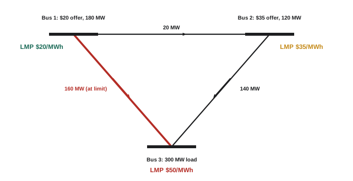
The result is surprising at first: the price at the load bus, $50/MWh, is higher than either generator's offer. Serving one more megawatt at bus 3 without overloading line 1-3 requires increasing the expensive bus 2 generator by 2 MW and decreasing the cheap bus 1 generator by 1 MW (because two-thirds of any bus 1 injection flows on the congested line), costing \(2 \times 35 - 20 = \$50\). Such counter-intuitive results are typical of meshed networks, where power flows on all parallel paths according to their impedances rather than along chosen routes.

Most North American wholesale markets, operated by independent system operators such as PJM, MISO, ERCOT, CAISO, NYISO, ISO-NE and the Alberta and Ontario operators (in different forms), clear day-ahead and real-time markets with security-constrained unit commitment and economic dispatch, paying generators and charging loads the LMP at their locations. The difference between prices at two locations is the congestion cost, which can be hedged with financial transmission rights. Price differences that persist signal where new transmission or generation would be most valuable, linking operations to planning (Lesson 12).