Power system structure

An electric power system is the largest and most complex machine ever built. It converts energy from fuel, falling water, wind, sunlight and nuclear fission into electricity, carries it hundreds of kilometres at hundreds of kilovolts, and delivers it to millions of customers at a few hundred volts, all while matching generation to consumption instant by instant, because the network itself stores almost no energy. Power systems analysis provides the models and calculations that engineers use to plan, operate and protect this machine: how voltages and power flows settle across the network, what happens when a line trips or a fault occurs, and how much new load, such as a data centre campus, the network can accept. This course builds those tools, starting from the circuit analysis of ELE-202 and ELE-203.

This lesson describes the structure of the system and the main concepts used throughout the course. The section at the end of this lesson sets out how the twelve lessons build from models of the components to load flow, control, stability, faults and planning.

From generation to the customer

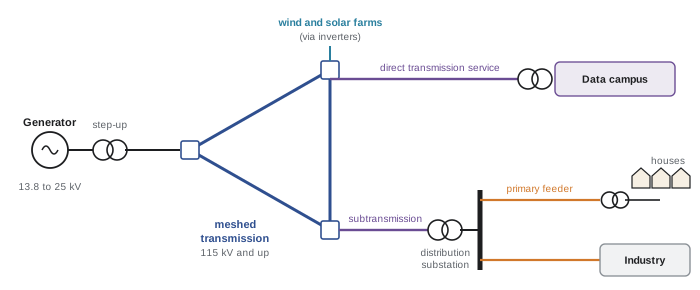
A power system has three functional layers:

• Generation: synchronous generators driven by steam, gas or hydro turbines produce three-phase power at 13.8 to 25 kV, and step-up transformers raise it to transmission voltage. Wind turbines, solar farms and batteries connect through power electronic inverters instead of rotating machines, a difference with growing consequences for system stability.
• Transmission: a meshed network of high-voltage and extra-high-voltage lines, typically 115 kV and above, carries bulk power over long distances and interconnects generating stations and load centres. Meshing gives multiple paths, so that the loss of one line does not interrupt supply. Subtransmission (roughly 34.5 to 138 kV) feeds distribution substations and large industrial customers.
• Distribution: substations step the voltage down to primary distribution levels, and radial feeders carry power through neighbourhoods, where pole-mounted or pad-mounted transformers reduce it again to the utilization voltage of buildings.

In Canada, common transmission voltages include 230, 345 and 500 kV, and Hydro-Québec operates a 735 kV network, one of the first in the world at that level, to bring power from northern hydroelectric stations to Montreal. Primary distribution is commonly 25 kV or 12.47 kV, and utilization voltages are 120/240 V single-phase for houses and 347/600 V or 120/208 V three-phase for commercial and industrial buildings.

Why transmit at high voltage?

For a given power, current is inversely proportional to voltage, and conductor losses are proportional to the square of the current. Raising the voltage by a factor of 10 reduces the current by 10 and the losses in the same conductor by 100. High voltage is what makes long-distance transmission economic, and the power transformer, which makes changing voltage cheap and efficient, is why AC won over DC at the end of the nineteenth century.

AC and HVDC

High-voltage direct current (HVDC) links convert AC to DC with power electronic converters, transmit it, and convert it back. Because they avoid the reactive effects of long AC lines (Lesson 4) and need only two conductors, HVDC links are economic for very long overhead lines (typically beyond 600 to 800 km), for submarine and underground cables beyond a few tens of kilometres, and for connecting grids that are not synchronized. Their converters also allow precise control of power flow.

Canadian examples include the Nelson River bipoles in Manitoba, the Hydro-Québec–New England multiterminal link, and the Maritime Link between Newfoundland and Nova Scotia.

Interconnections and system operation

Neighbouring utilities connect their networks so that they can share reserves, trade energy and help one another in emergencies. All generators in an AC interconnection rotate in synchronism at the same electrical frequency, so an interconnection is effectively one machine.

North America has four major AC interconnections: the Eastern, the Western, Texas (ERCOT) and Québec, linked to one another only through HVDC ties. Canadian provinces belong to the Eastern (Ontario, Manitoba, Saskatchewan, the Maritimes) or Western (British Columbia, Alberta) interconnections, apart from Québec, which forms its own. System operators such as Ontario's Independent Electricity System Operator (IESO), the Alberta Electric System Operator (AESO) and the provincial utilities balance supply and demand, and the North American Electric Reliability Corporation (NERC) sets reliability standards that are made mandatory by provincial regulators.

Balancing generation and load

Because the network stores almost no energy, any mismatch between generation and load is supplied from, or absorbed into, the kinetic energy of rotating generators and motors, changing their speed and hence the system frequency. The relationship is the swing equation for the aggregate system:

where \(H\) is the inertia constant (stored kinetic energy at rated speed divided by rated power, typically 2 to 9 seconds for synchronous generators), \(P_m\) mechanical input power and \(P_e\) electrical output. When a large generator trips, frequency starts to fall at a rate set by the system inertia. Within seconds, governors on other units increase their output (primary frequency response, proportional to the frequency deviation through droop, as in DCE-340); within minutes, automatic generation control restores frequency to 60 Hz and scheduled interchange between areas (secondary control); then operators redispatch generation (tertiary control). If frequency falls too far, under-frequency load shedding relays disconnect blocks of customers to save the rest of the system.

Reliability criteria

Transmission systems are planned and operated to the N−1 criterion: the system must remain within thermal, voltage and stability limits after the loss of any single element, such as a line, transformer or generator, and then be readjusted to withstand the next contingency. Some critical facilities are planned for N−1−1 or for credible multiple contingencies, such as a tower carrying two circuits collapsing. Load flow and fault studies (Lessons 6, 9 and 10) are the tools used to check these criteria, and interconnection studies for a new generator or large load, such as a data centre requesting 300 MW, run the same analyses on the planned future network.

Loads

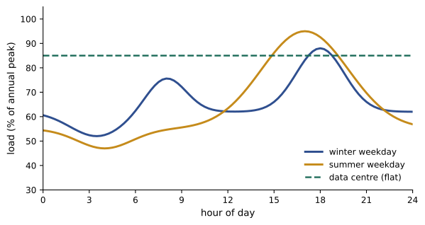
Load varies through the day and the year, driven by weather, working hours and lighting. The load curve shows demand against time; its peak sets the capacity the system must supply, and its shape sets how hard the rest of the fleet must work.

• Load factor: average load divided by peak load over a period. A data centre runs at a load factor of 0.8 to 0.9; a residential feeder may be near 0.4.
• Diversity factor: the sum of individual customers' peak demands divided by the coincident peak of the group, always at least 1. Because customers do not peak at the same time, a feeder or transformer can serve more customers than the sum of their peaks would suggest.
• Demand factor: maximum demand divided by connected load, the principle behind the dwelling load calculations of ELEC-130.

Load characteristics

In power flow studies, loads are represented by how their power varies with voltage. Constant-power loads (motors with drives, switch-mode power supplies, data centre UPSs) draw the same power regardless of voltage, so their current rises as voltage falls, which can aggravate voltage collapse. Constant-impedance loads (resistive heaters, incandescent lighting) draw power proportional to voltage squared, and constant-current loads lie in between. Real loads are combinations, often modelled by the ZIP model, a weighted sum of the three.

Single-line diagrams and three-phase power

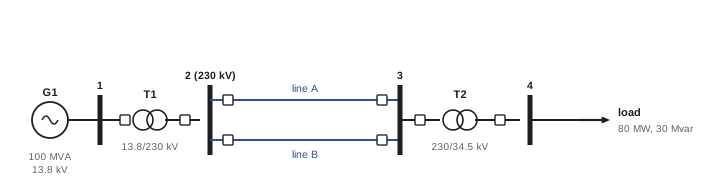
Balanced three-phase systems are analysed per phase, as in ELE-203, and drawn as single-line (one-line) diagrams, in which one line represents all three phases and standard symbols represent generators, transformers, breakers, buses, lines and loads. The single-line diagram, annotated with ratings and impedances, is the starting point of every study in this course.

Recall that for a balanced three-phase system, complex power is

where \(P\) in watts is real power and \(Q\) in vars is reactive power, positive for inductive (lagging) loads. Reactive power does no net work but must flow back and forth to sustain magnetic and electric fields; it causes voltage drops and losses, and is supplied locally where possible by capacitor banks, synchronous condensers, static var compensators and inverters. A central theme of power systems is that real power flow is governed mainly by voltage angle differences, while reactive power flow is governed mainly by voltage magnitude differences, as Lesson 4 shows.

How this course is organized

The twelve lessons move from the components of the system to its analysis, control and planning:

• Lesson 1 (this lesson): structure of the power system, interconnections, loads and three-phase power.
• Lesson 2: per-unit analysis and transformer models.
• Lesson 3: synchronous generators, their capability and dynamic reactances.
• Lesson 4: transmission line parameters, models, loadability and compensation.
• Lesson 5: reactive power, voltage control and voltage stability.
• Lesson 6: load flow by Gauss-Seidel, Newton-Raphson, fast decoupled and DC methods.
• Lesson 7: economic dispatch, unit commitment, optimal power flow and locational marginal prices.
• Lesson 8: transient and small-signal stability.
• Lesson 9: fault analysis, symmetrical components and grounding.
• Lesson 10: unbalanced faults in networks, transformer connections and short-circuit standards.
• Lesson 11: frequency control, AGC, reserves and underfrequency load shedding.
• Lesson 12: planning, the integration of new resources and loads, and a system study project.