
ELE-380 · Lesson 11 of 12 · 33 min
Frequency control and system balancing
Electrical energy is produced at the instant it is consumed, so generation must match load continuously. Frequency is the indicator of that balance across a whole interconnection: when generation exceeds load, the surplus accelerates every synchronous machine and frequency rises; when load exceeds generation, frequency falls. Keeping frequency within a narrow band, typically within ±0.05 Hz of 60 Hz in normal operation, requires a layered set of controls acting from fractions of a second to hours. This lesson follows a sudden loss of generation through those layers: inertial response, primary control by governors, secondary control by automatic generation control between balancing areas, and tertiary control and reserves, and then examines the challenge of falling inertia as inverter-based resources replace synchronous machines, and the role of underfrequency load shedding as the last line of defence.
Inertial response
In the first moments after a generator trips, nothing has yet acted to replace its output. The power deficit is supplied by the kinetic energy stored in the rotating masses of all synchronous machines (and synchronous motors), which slow down together. Summing the swing equations of Lesson 8 over the whole system gives the initial rate of change of frequency (RoCoF):
where \(\Delta P\) is the lost generation, \(S_{\text{sys}}\) the total rating of online synchronous machines and \(H_{\text{sys}}\) their combined inertia constant. RoCoF matters because every subsequent control needs time to act; the faster frequency falls, the deeper it goes before those controls arrest it.
Worked problem
Rate of change of frequency
An interconnection has 60,000 MVA of online synchronous generation with an average \(H\) of 4 s. A 1,200 MW unit trips. What is the initial RoCoF? How would it change if half the synchronous generation were replaced by inverter-based resources without inertia?
Show solution
- Stored energy: \(4 \times 60{,}000 = 240{,}000\) MW·s.
- RoCoF: \(-1{,}200 \times 60/(2 \times 240{,}000) = -0.15\) Hz/s.
- With half the inertia: \(-0.30\) Hz/s.
Answer: An initial fall of 0.15 Hz/s, doubling to 0.30 Hz/s with half the inertia. Small isolated systems with high renewable shares, such as islands, can see RoCoF above 1 Hz/s, which may itself trip generator protection relays set on RoCoF.
Primary control: governors and droop
Within a few seconds, turbine governors respond to the falling speed by opening valves or gates. Each governor has a droop characteristic: its output rises in proportion to the frequency drop. A droop \(R\) of 5% means that a 5% fall in frequency (3 Hz at 60 Hz) would drive the unit from zero to full output:
Droop lets many governors share a change in load stably, in proportion to their ratings, without fighting each other, which an isochronous (zero-droop) controller on every unit would do. Typical droops are 4% to 5%, with intentional deadbands of about ±0.036 Hz so that governors do not respond to normal small fluctuations.
Load also helps: motors slow down and draw less power when frequency falls, an effect called load damping, typically 1% to 2% of load per 1% change in frequency. The combined steady-state response of governors and load defines the frequency response characteristic \(\beta\) of the interconnection, in MW per 0.1 Hz:
Worked problem
Settling frequency
An interconnection carries 50,000 MW of load. Generators totalling 40,000 MW of capacity provide governor response with 5% droop; the rest are at maximum output or have their governors blocked. Load damping is 1.5% per 1% of frequency. A 1,000 MW unit trips. Find the settling frequency after primary control.
Show solution
- Governors: \(40{,}000/(0.05 \times 60) = 13{,}333\) MW/Hz.
- Load: \(1.5 \times 50{,}000/60 = 1{,}250\) MW/Hz.
- \(\beta = 14{,}583\) MW/Hz (1,458 MW per 0.1 Hz). \(\Delta f = -1{,}000/14{,}583 = -0.069\) Hz.
Answer: Frequency settles about 0.07 Hz low, at 59.93 Hz, with governors supplying about 914 MW and load reduction the other 86 MW. In practice many units have blocked or sluggish governors, and actual frequency response in North American interconnections is lower than such calculations suggest, which led to NERC's frequency response standard (BAL-003).
The lowest point of the frequency excursion, the nadir, occurs a few seconds after the event, when governor response catches up with the deficit. It is deeper than the settling frequency, because turbines respond with lags of several seconds (steam reheat units are slow, gas turbines and hydro units faster but with their own dynamics). The nadir must stay above the first stage of underfrequency load shedding with margin.
Secondary control: automatic generation control
Primary control arrests the fall but leaves frequency below 60 Hz, and the replacement power comes from governors all over the interconnection, so flows between regions deviate from their schedules. Secondary control restores both. The interconnection is divided into balancing authority areas, each responsible for matching its own generation to its own load plus scheduled interchange. Each area computes its area control error (ACE) every few seconds:
where \(NI_A\) and \(NI_S\) are actual and scheduled net interchange (exports positive), \(F_A\) and \(F_S\) actual and scheduled frequency, and \(B\) the area's frequency bias in MW/0.1 Hz (negative by convention), set close to the area's own frequency response. Automatic generation control (AGC) adjusts the set points of participating units to drive ACE toward zero over several minutes. The bias term is the key: for an event outside the area, the area's governor response increases its exports, but the frequency term cancels that, so its ACE stays near zero and AGC leaves its governors' help in place; for an event inside the area, both terms point the same way and AGC raises generation to replace the loss.
Worked problem
Who replaces the lost unit?
Two areas are interconnected. Area A has bias \(-500\) MW/0.1 Hz and area B \(-1{,}000\) MW/0.1 Hz, each matching its frequency response. A 600 MW unit trips in area A. Frequency settles 0.04 Hz low before AGC acts, and area B's governors raise its exports to A by 400 MW. Compute each area's ACE.
Show solution
- Area A: interchange deviation \(-400\) MW (it imports 400 MW more). Frequency term: \(-10 \times (-500) \times (-0.04) = -200\) MW. ACE \(= -400 - 200 = -600\) MW.
- Area B: interchange deviation \(+400\) MW. Frequency term: \(-10 \times (-1{,}000) \times (-0.04) = -400\) MW. ACE \(= 400 - 400 = 0\).
Answer: Area A's ACE is −600 MW, exactly the lost unit, so its AGC raises generation by 600 MW; area B's ACE is zero, so it takes no action and its governors return to normal as frequency recovers. Each area replaces its own losses.
Performance standards (NERC BAL-001 in North America) require each area to keep ACE small on average and to recover from large disturbances within 15 minutes. Small systems may implement AGC with a few hydro or gas units; large ones dispatch hundreds of units, and modern markets combine AGC with five-minute economic dispatch (Lesson 7) so that regulation is provided at least cost.
Tertiary control and reserves
Tertiary control restores the reserves used by primary and secondary control, by redispatching or starting units within 10 to 30 minutes, ready for the next event. Operators carry several categories of reserve:
| Reserve | Purpose | Response time | Typical providers |
|---|---|---|---|
| Primary frequency response | arrest frequency after a contingency | seconds | governors, batteries, fast load response |
| Regulation | follow minute-to-minute imbalances via AGC | seconds to minutes | gas, hydro, batteries |
| Contingency (spinning) | replace the largest credible loss | within 10 minutes, synchronized | part-loaded units, batteries |
| Contingency (non-spinning) | replace a loss with quick-start units | within 10 to 30 minutes | combustion turbines, interruptible load |
| Ramping or flexibility | cover forecast errors and steep ramps in net load | 5 to 60 minutes | flexible thermal plants, storage, demand response |
The amount of contingency reserve is set by the largest credible loss, often the largest unit or the largest import line. With high shares of wind and solar, uncertainty in their output adds to reserve needs, and the steep evening ramp in net load (load minus solar output, the so-called duck curve) requires flexible capacity able to increase output by thousands of megawatts in a few hours.
Simulating a frequency event
import numpy as np

f0 = 60.0
def event(H, loss=0.02, R=0.05, D=1.0, Tg=1.5, share=0.4, agc=False, ffr=0.0, t_end=300.0, dt=0.01):
    """Per unit on system base: lose a fraction loss of generation at t = 0. Returns RoCoF, nadir, settling frequency."""
    df, Pg, Pffr, integ = 0.0, 0.0, 0.0, 0.0
    nadir, rocof = 0.0, None
    for step in range(int(t_end / dt)):
        Pload_change = D * df                           # load falls as frequency falls (D in pu MW per pu Hz)
        acc = (Pg + Pffr - loss - Pload_change) / (2 * H)   # d(df)/dt in pu Hz per second
        if rocof is None: rocof = acc * f0
        target = -share * df / R - (0.5 * integ if agc else 0.0)   # droop on the responsive share of capacity, plus AGC
        Pg += (target - Pg) * dt / Tg                   # turbine-governor lag
        Pffr = ffr if df * f0 < -0.15 else Pffr          # fast frequency response triggers below 59.85 Hz
        integ += df * dt
        df += acc * dt
        nadir = min(nadir, df)
    return rocof, f0 * (1 + nadir), f0 * (1 + df)

for label, kw in (("H = 5 s", dict(H=5.0)), ("H = 2.5 s", dict(H=2.5)), ("H = 2.5 s + 1% fast response", dict(H=2.5, ffr=0.01)),
                  ("H = 5 s with AGC", dict(H=5.0, agc=True))):
    rocof, nad, fin = event(**kw)
    print(f"{label:30s}: initial RoCoF {rocof:+.3f} Hz/s, nadir {nad:.3f} Hz, after 300 s {fin:.3f} Hz")
beta = 0.4 / 0.05 + 1.0
print(f"steady-state deviation without AGC: {-0.02 / beta * f0:.3f} Hz (from the frequency response characteristic)")H = 5 s : initial RoCoF -0.120 Hz/s, nadir 59.819 Hz, after 300 s 59.867 Hz H = 2.5 s : initial RoCoF -0.240 Hz/s, nadir 59.770 Hz, after 300 s 59.867 Hz H = 2.5 s + 1% fast response : initial RoCoF -0.240 Hz/s, nadir 59.843 Hz, after 300 s 59.933 Hz H = 5 s with AGC : initial RoCoF -0.120 Hz/s, nadir 59.824 Hz, after 300 s 60.000 Hz steady-state deviation without AGC: -0.133 Hz (from the frequency response characteristic)
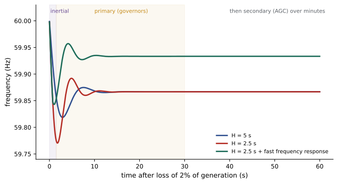
Halving inertia doubles the initial RoCoF and deepens the nadir, while leaving the settling frequency unchanged, because that depends only on droop and load damping. Fast frequency response from batteries, triggered when frequency falls 0.15 Hz, more than makes up for the lost inertia. AGC returns frequency to 60 Hz over a few minutes.
Low inertia and fast frequency response
As inverter-based wind, solar and batteries displace synchronous plants, system inertia falls, especially at times of low load and high renewable output. Operators in systems such as ERCOT, Great Britain, Ireland and Australia monitor inertia in real time and set minimum inertia levels, constraining how much synchronous generation can be turned off. Responses include:
- Fast frequency response: batteries and other inverter-based resources inject power within a few hundred milliseconds of detecting a frequency drop, much faster than any governor. ERCOT's market includes a fast frequency response product, and Great Britain's dynamic containment service procures similar response.
- Synthetic inertia: inverters, including wind turbines drawing on rotor kinetic energy, respond in proportion to RoCoF.
- Grid-forming inverters: behaving as voltage sources, they respond inherently to frequency changes like synchronous machines.
- Synchronous condensers, some with flywheels, add real inertia (Lesson 3).
- Raising RoCoF withstand capabilities of generators and their protection, so that units do not trip during fast transients.
- Demand response: interruptible industrial loads and, increasingly, data centres that can reduce consumption quickly on frequency signals.
Underfrequency load shedding
If a disturbance exceeds the reserves, for example when an interconnection separates into islands with a large generation deficit, frequency continues to fall. Below about 57 to 58.5 Hz, steam turbine blades risk damaging resonance and generator protection begins to trip units, which would accelerate the collapse. Underfrequency load shedding (UFLS) relays automatically disconnect blocks of load in stages, for example 5% to 10% of load at each of several thresholds starting near 59.3 Hz in many North American regions, to restore balance. The stages are coordinated with generator underfrequency protection, so that load is shed before generators trip, and they are designed for credible islanding scenarios with deficits of up to 25% to 30%.
Worked problem
Islanding and load shedding
A region separates from the interconnection while importing 1,500 MW, leaving 8,500 MW of generation to supply 10,000 MW of load. Its UFLS program sheds 6% of load at each of five stages. How many stages must operate, at a minimum, to balance generation and load, ignoring governor response and load damping?
Show solution
- Deficit: 1,500 MW, or 15% of load.
- Each stage sheds 600 MW. Two stages shed 1,200 MW, still 300 MW short; three shed 1,800 MW.
Answer: Three stages (18% of load). The 300 MW excess shed would push frequency above 60 Hz until governors reduce output; in practice load damping and governors also help, so the program is tuned with dynamic simulations to avoid both under- and overshoot.
Restoring the shed load must be done gradually as generation is brought up, coordinating with the system operator. Electric clocks once kept time by counting cycles, and accumulated time error is still corrected by small offsets in scheduled frequency, though its practical importance has diminished.
Common mistakes
MistakeAssuming governors can stop the initial frequency fall.
InsteadOnly inertia acts in the first second; RoCoF depends on stored kinetic energy.
MistakeRunning governors isochronously on many units.
InsteadUse droop so that units share changes stably; restore frequency with AGC.
MistakeSetting frequency bias far from the area's actual response.
InsteadMatch bias to frequency response so each area replaces only its own losses.
MistakeCounting nameplate capacity of units with blocked governors as primary response.
InsteadOnly units with active governors and headroom contribute.
MistakeIgnoring falling inertia as renewables grow.
InsteadMonitor inertia, procure fast frequency response, and use grid-forming resources.
Summary and key terms
- Frequency reflects the balance of generation and load across an interconnection.
- Inertia sets the initial rate of change of frequency after a loss.
- Governor droop shares the response and determines the settling frequency with load damping.
- AGC uses area control error with frequency bias to restore frequency and scheduled interchange, so each area replaces its own losses.
- Reserves of several speeds cover regulation, contingencies and ramps.
- Low inertia is countered by fast frequency response, grid-forming inverters and condensers; underfrequency load shedding is the last defence.
- RoCoF
- Rate of change of frequency, set initially by the power imbalance and system inertia.
- Droop
- The percentage frequency change that drives a governor from zero to full output.
- Load damping
- The reduction of load power as frequency falls.
- Frequency response characteristic
- The MW change per 0.1 Hz from governors and load combined.
- Nadir
- The lowest frequency reached after a loss of generation.
- Balancing authority
- The entity balancing generation, load and interchange in an area.
- Area control error
- Interchange deviation minus frequency bias times frequency deviation.
- AGC
- Automatic generation control, adjusting unit set points to drive ACE to zero.
- Fast frequency response
- Very fast injection of power, mostly from inverter-based resources, after a frequency drop.
- Underfrequency load shedding
- Automatic disconnection of load blocks at set frequency thresholds.
Practice problems
Work each problem on paper first, then reveal the answer to check.
RoCoF for losing 500 MW with 100,000 MW·s of stored energy at 60 Hz?
Show answer
\(-500 \times 60/200{,}000 = -0.15\) Hz/s.
A 400 MW unit with 5% droop: output change for a 0.1 Hz drop at 60 Hz?
Show answer
\(400 \times 0.1/3 = 13.3\) MW.
Two units of 300 and 600 MW with equal droop share a 90 MW increase. Each provides?
Show answer
30 and 60 MW.
\(\beta = 2{,}000\) MW/0.1 Hz; a 1,000 MW loss gives what settling deviation?
Show answer
−0.05 Hz.
Why is the nadir lower than the settling frequency?
Show answer
Governors and turbines respond with lags of several seconds.
ACE for an area exporting 50 MW less than scheduled with \(B = -200\) MW/0.1 Hz and \(\Delta f = 0\)?
Show answer
−50 MW.
What does the frequency bias term achieve?
Show answer
It cancels an area's governor support for external events so only the area with the loss acts.
Name two categories of contingency reserve.
Show answer
Spinning and non-spinning.
Why are minimum inertia limits set in some systems?
Show answer
To keep RoCoF and nadir within limits after the largest contingency.
A 2,000 MW deficit on 12,000 MW of load with 5% UFLS stages: stages needed?
Show answer
4 stages (2,400 MW); 3 stages shed only 1,800 MW.
Lesson quiz · 5 questions
Score 60% or more to complete this lesson.
Create a free account to save your progress, take quizzes and earn a certificate.