
ELE-380 · Lesson 6 of 12 · 32 min
Load flow
Load flow (or power flow) analysis answers the most basic question about a power system in steady state: given the loads and the generators' outputs and voltage settings, what are the voltages at every bus and the power flows on every line and transformer? It is the most frequently run calculation in power engineering. Planners use it to check that the network will stay within limits as loads grow and new generators or data centres connect; operators run it continuously in control centres, together with contingency analysis, to make sure that the loss of any element will not cause overloads or voltage problems. This lesson formulates the load flow problem, builds the bus admittance matrix, develops the Gauss-Seidel and Newton-Raphson solution methods and the fast decoupled and DC approximations, and shows how load flow supports voltage control and contingency analysis.
The bus admittance matrix
The network of lines and transformers, represented by their per-unit π equivalents (Lessons 2 and 4), is linear. Nodal analysis from ELE-202 relates the injected currents at the buses to the bus voltages through the bus admittance matrix:
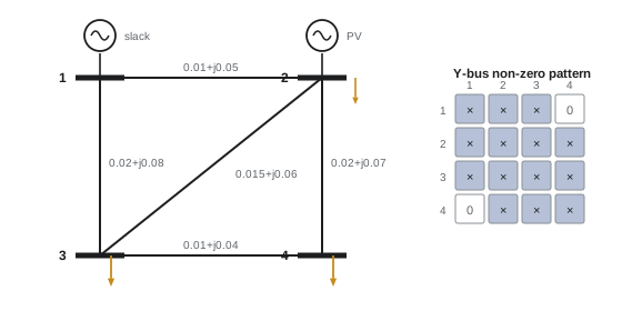
It is built by inspection: each diagonal element \(Y_{ii}\) is the sum of all admittances connected to bus \(i\), including half the charging susceptance of each line and any shunt elements; each off-diagonal element \(Y_{ij}\) is the negative of the series admittance between buses \(i\) and \(j\), and zero if they are not directly connected. Because each bus connects to only a few others, \(Y_{\mathrm{bus}}\) is extremely sparse: a 10,000-bus network might have only three or four non-zero entries per row, and sparse matrix techniques make large studies fast.
The load flow equations
The complex power injected at bus \(i\) is \(S_i = V_iI_i^*\). Substituting the nodal equations gives the power flow equations:
Writing \(V_i = |V_i|\angle\theta_i\) and \(Y_{ik} = G_{ik} + jB_{ik}\), the real and imaginary parts are
with \(\theta_{ik} = \theta_i - \theta_k\). Each bus has four quantities, \(P\), \(Q\), \(|V|\) and \(\theta\); two are specified and two are found. Buses are classified accordingly:
| Bus type | Specified | Unknown | Typical example |
|---|---|---|---|
| Slack (swing, reference) | \(|V|\) and \(\theta = 0\) | \(P\), \(Q\) | One large generator; supplies the losses, which are not known in advance |
| PV (generator) | \(P\) and \(|V|\) | \(Q\), \(\theta\) | Generators with voltage regulators, synchronous condensers, STATCOMs |
| PQ (load) | \(P\) and \(Q\) | \(|V|\), \(\theta\) | Load buses and buses with no generation |
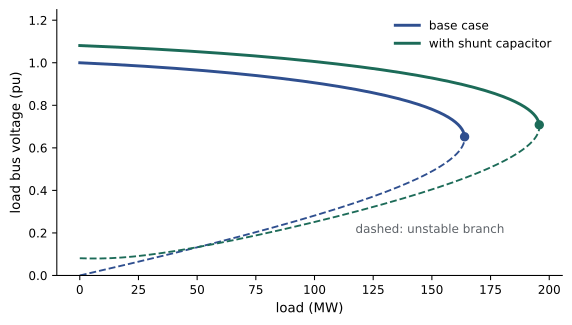
The equations are non-linear in the voltages, so there is no closed-form solution; they are solved by iteration. A load flow may also have no solution at all, when the loads exceed what the network can deliver; this corresponds physically to voltage collapse, and the point at which solutions cease to exist is the voltage stability limit.
Gauss-Seidel method
The earliest computer method rearranges the equation for each PQ bus to give its voltage in terms of the others:
and sweeps through the buses repeatedly, using each new value immediately. For PV buses, \(Q_i\) is first estimated from the current voltages and the voltage magnitude is reset to its setpoint after each update. Gauss-Seidel is simple and needs little memory, but its convergence slows dramatically as networks grow, often needing hundreds of iterations, and it is now used mainly for small systems and to provide starting values.
Newton-Raphson method
Newton-Raphson linearizes the equations around the current estimate and solves for a correction. The unknowns are the angles of all non-slack buses and the voltage magnitudes of the PQ buses; the equations are the mismatches between scheduled and calculated power, \(\Delta P_i = P_i^{\mathrm{sch}} - P_i(\theta, |V|)\) at PV and PQ buses and \(\Delta Q_i\) at PQ buses. Each iteration solves
for the corrections, updates the voltages, and repeats. The matrix of partial derivatives is the Jacobian; it is sparse with the same pattern as \(Y_{\mathrm{bus}}\), and is recomputed every iteration. Newton-Raphson converges quadratically near the solution, roughly doubling the number of correct digits each iteration, and typically reaches a mismatch below \(10^{-6}\) pu in three to five iterations regardless of system size. It is the standard method in commercial software.
import numpy as np

# lines: from, to, R, X, total charging B (pu on 100 MVA)
lines = [(1, 2, 0.010, 0.050, 0.040), (1, 3, 0.020, 0.080, 0.040), (2, 3, 0.015, 0.060, 0.030),
         (2, 4, 0.020, 0.070, 0.030), (3, 4, 0.010, 0.040, 0.020)]
n = 4
Y = np.zeros((n, n), complex)
for f, t, R, X, B in lines:
    i, j = f - 1, t - 1
    y = 1 / complex(R, X)
    Y[i, i] += y + 0.5j * B; Y[j, j] += y + 0.5j * B
    Y[i, j] -= y; Y[j, i] -= y

# bus data: type (0 slack, 1 PV, 2 PQ), |V| setpoint, P generation, P load, Q load
btype = np.array([0, 1, 2, 2])
Vset = np.array([1.02, 1.01, 1.0, 1.0])
Pg = np.array([0.0, 1.0, 0.0, 0.0])
Pd = np.array([0.0, 0.2, 1.2, 0.9]); Qd = np.array([0.0, 0.1, 0.5, 0.35])
Psch, Qsch = Pg - Pd, -Qd

V = Vset.astype(complex)
pv_pq = np.where(btype > 0)[0]; pq = np.where(btype == 2)[0]
for it in range(10):
    S = V * np.conj(Y @ V)
    mis = np.concatenate([Psch[pv_pq] - S.real[pv_pq], Qsch[pq] - S.imag[pq]])
    print(f"iteration {it}: largest mismatch = {np.abs(mis).max():.2e} pu")
    if np.abs(mis).max() < 1e-8:
        break
    Ibus = Y @ V
    dS_dVa = 1j * np.diag(V) @ np.conj(np.diag(Ibus) - Y @ np.diag(V))
    dS_dVm = np.diag(V) @ np.conj(Y @ np.diag(V / abs(V))) + np.conj(np.diag(Ibus)) @ np.diag(V / abs(V))
    J = np.block([[dS_dVa.real[np.ix_(pv_pq, pv_pq)], dS_dVm.real[np.ix_(pv_pq, pq)]],
                  [dS_dVa.imag[np.ix_(pq, pv_pq)], dS_dVm.imag[np.ix_(pq, pq)]]])
    dx = np.linalg.solve(J, mis)
    Va = np.angle(V); Vm = abs(V)
    Va[pv_pq] += dx[:len(pv_pq)]; Vm[pq] += dx[len(pv_pq):]
    V = Vm * np.exp(1j * Va)

S = V * np.conj(Y @ V)
print("bus  |V| pu  angle deg   P inj MW  Q inj Mvar")
for k in range(n):
    print(f"{k + 1:3d}  {abs(V[k]):.4f}  {np.degrees(np.angle(V[k])):8.3f}  {100 * S[k].real:9.1f}  {100 * S[k].imag:9.1f}")
loss = 0
print("line   P from MW  Q from Mvar  loss MW")
for f, t, R, X, B in lines:
    i, j = f - 1, t - 1
    y = 1 / complex(R, X)
    Sij = V[i] * np.conj((V[i] - V[j]) * y + V[i] * 0.5j * B)
    Sji = V[j] * np.conj((V[j] - V[i]) * y + V[j] * 0.5j * B)
    loss += (Sij + Sji).real
    print(f"{f}-{t}   {100 * Sij.real:8.1f}  {100 * Sij.imag:10.1f}  {100 * (Sij + Sji).real:7.2f}")
print(f"total losses {100 * loss:.2f} MW; slack generation {100 * S[0].real:.1f} MW")iteration 0: largest mismatch = 1.10e+00 pu iteration 1: largest mismatch = 3.09e-02 pu iteration 2: largest mismatch = 6.31e-05 pu iteration 3: largest mismatch = 2.64e-10 pu bus |V| pu angle deg P inj MW Q inj Mvar 1 1.0200 0.000 133.6 36.4 2 1.0100 -1.410 80.0 46.8 3 0.9823 -3.355 -120.0 -50.0 4 0.9770 -3.853 -90.0 -35.0 line P from MW Q from Mvar loss MW 1-2 52.8 8.4 0.28 1-3 80.8 28.0 1.43 2-3 64.0 30.1 0.75 2-4 68.5 27.8 1.09 3-4 22.7 6.4 0.06 total losses 3.60 MW; slack generation 133.6 MW
The mismatch falls from 1.1 pu to \(10^{-10}\) in three iterations, the hallmark of quadratic convergence. The generator at bus 2 holds its terminal at 1.01 pu by supplying 46.8 Mvar net of its local load; the load buses settle at 0.98 pu, and voltage angles decrease from the slack toward the loads, showing real power flowing "downhill" in angle. The slack generator supplies 133.6 MW: the 230 MW of load, less the 100 MW from bus 2, plus 3.6 MW of losses that could only be found by solving the load flow.
Worked problem
Building Y-bus
For the four-bus network, find \(Y_{12}\) and \(Y_{11}\). Line 1-2 has \(z = 0.01 + j0.05\) pu and total charging \(B = 0.04\); line 1-3 has \(z = 0.02 + j0.08\) and \(B = 0.04\).
Show solution
- Line 1-2: \(y_{12} = 1/(0.01 + j0.05) = 3.846 - j19.231\).
- Line 1-3: \(y_{13} = 1/(0.02 + j0.08) = 2.941 - j11.765\).
- \(Y_{12} = -y_{12} = -3.846 + j19.231\).
- \(Y_{11} = y_{12} + y_{13} + j(0.04 + 0.04)/2 = 6.787 - j30.956\).
Answer: \(Y_{12} = -3.85 + j19.23\) and \(Y_{11} = 6.79 - j30.96\) pu. \(Y_{14} = 0\) because buses 1 and 4 are not directly connected.
Fast decoupled load flow
At transmission level, \(X \gg R\) and angle differences across lines are small, so real power depends strongly on angles and weakly on voltage magnitudes, while reactive power depends strongly on magnitudes and weakly on angles (as in Lesson 4). The fast decoupled method exploits this by neglecting the off-diagonal blocks of the Jacobian and approximating the diagonal blocks by constant matrices \(B'\) and \(B''\) built from line reactances:
The constant matrices are factorized once, so each iteration is very cheap. Convergence is linear rather than quadratic and needs more iterations, but the total time is often less, which makes the method popular for contingency screening, where thousands of cases are solved.
DC load flow
Going further, assume all voltage magnitudes are 1.0 pu, resistances are negligible and angle differences are small, so \(\sin\theta_{ik} \approx \theta_{ik}\). Then the flow on a line is simply
a linear system, like a DC resistive circuit with angles playing the role of voltages and reactances the role of resistances. The DC load flow ignores reactive power, voltage magnitudes and losses, but it gives real power flows to within a few percent on transmission networks, needs no iteration, and is the basis of electricity market models (locational marginal prices), transmission expansion planning and fast contingency screening.
import numpy as np

lines = [(1, 2, 0.050), (1, 3, 0.080), (2, 3, 0.060), (2, 4, 0.070), (3, 4, 0.040)]
rating = {(1, 2): 150, (1, 3): 150, (2, 3): 110, (2, 4): 120, (3, 4): 80}   # MW
P = np.array([0.0, 0.8, -1.2, -0.9])          # net injections (pu); bus 1 is the slack

def dc_flow(active):
    n = 4
    B = np.zeros((n, n))
    for f, t, X in active:
        i, j = f - 1, t - 1
        B[i, i] += 1 / X; B[j, j] += 1 / X; B[i, j] -= 1 / X; B[j, i] -= 1 / X
    theta = np.zeros(n)
    theta[1:] = np.linalg.solve(B[1:, 1:], P[1:])   # slack angle = 0
    return {(f, t): 100 * (theta[f - 1] - theta[t - 1]) / X for f, t, X in active}

base = dc_flow(lines)
print("base case flows (MW):", {f"{k[0]}-{k[1]}": float(round(v, 1)) for k, v in base.items()})
print("N-1 contingency analysis:")
for out in lines:
    flows = dc_flow([l for l in lines if l != out])
    worst = max(flows, key=lambda k: abs(flows[k]) / rating[k])
    load = abs(flows[worst]) / rating[worst]
    flag = "OVERLOAD" if load > 1 else "ok"
    print(f"  outage of {out[0]}-{out[1]}: worst line {worst[0]}-{worst[1]} at {abs(flows[worst]):6.1f} MW "
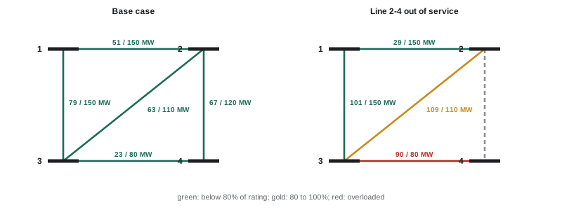
f"({load:5.0%} of rating) {flag}")base case flows (MW): {'1-2': 50.7, '1-3': 79.3, '2-3': 63.4, '2-4': 67.3, '3-4': 22.7}
N-1 contingency analysis:
outage of 1-2: worst line 1-3 at 130.0 MW ( 87% of rating) ok
outage of 1-3: worst line 2-3 at 114.7 MW ( 104% of rating) OVERLOAD
outage of 2-3: worst line 2-4 at 101.7 MW ( 85% of rating) ok
outage of 2-4: worst line 3-4 at 90.0 MW ( 112% of rating) OVERLOAD
outage of 3-4: worst line 2-4 at 90.0 MW ( 75% of rating) okThe DC flows agree with the full AC solution within about 2 MW (for example 79.3 MW against 80.8 MW on line 1-3), because losses and voltage magnitudes are ignored. The contingency screen shows why N−1 matters: the base case is comfortable, but losing line 1-3 overloads line 2-3, and losing line 2-4 forces all the power for bus 4 through line 3-4, overloading it by 12%. Remedies include re-dispatching generation (raising output at bus 2 relieves both), upgrading the overloaded lines, adding a line, or a special protection scheme that sheds load after the outage.
Voltage control in load flow
Realistic load flows include the devices that regulate voltage:
- Generator reactive limits: a PV bus holds its voltage only while its reactive output stays within the generator's capability. If the solution requires more, the bus is converted to a PQ bus with \(Q\) fixed at the limit, and its voltage is allowed to fall.
- Transformer taps: on-load tap changers adjust the off-nominal ratio between iterations to hold a target voltage at a bus, within the tap range.
- Switched shunt capacitors and reactors are switched in or out to keep voltages within a band.
- Phase-shifting transformers adjust angles to control real power flow on a corridor.
Because these controls interact, load flow programs alternate between solving the network and adjusting the controls until both settle.
Worked problem
A PV bus hitting its limit
A generator bus is set to hold 1.03 pu, but the solution requires 180 Mvar from a unit whose maximum reactive output is 150 Mvar. What does the load flow do, and what happens to voltages?
Show solution
- The bus is switched from PV to PQ with \(Q = 150\) Mvar (net of any local load).
- The load flow is re-solved; with less reactive support, the bus voltage falls below 1.03 pu, and nearby load buses also fall.
Answer: The voltage at the generator bus falls below its setpoint, possibly to around 1.00 pu or lower, and neighbouring voltages drop. If they fall below limits, additional reactive support (capacitors, a STATCOM) or a different generator dispatch is needed. Reaching reactive limits one after another is a classic path to voltage collapse.
Using load flow
Load flow studies support most planning and operating decisions:
- Interconnection studies for new generators and large loads, such as a data centre campus, test whether the network can supply the new load under N−1 conditions, and identify the upgrades the customer must fund.
- Transfer capability studies find how much power can move between regions before a limit is reached.
- Voltage stability studies trace PV curves (receiving voltage against load) by solving a sequence of load flows with increasing load until no solution exists, giving the margin to collapse.
- Operators run a state estimator, which fits a load flow solution to thousands of real-time measurements, then contingency analysis on the estimated state every few minutes, and optimal power flow, which adds an objective such as minimum generation cost subject to all limits.
Lesson 7 adds costs and limits to load flow to obtain economic dispatch and optimal power flow, and Lesson 12 applies contingency analysis to a planning study.
Common mistakes
MistakeOmitting the slack bus or specifying P at every bus.
InsteadLosses are unknown until solved; one slack bus balances them.
MistakeIgnoring generator reactive limits.
InsteadConvert PV buses to PQ at their limits; otherwise voltages are unrealistically supported.
MistakeUsing DC load flow to study voltages or reactive power.
InsteadDC load flow gives only approximate real power flows; use AC load flow for voltages.
MistakeTreating a non-converging load flow as a numerical nuisance.
InsteadIt may mean the operating point does not exist: the system is beyond its voltage stability limit.
MistakeChecking only the base case.
InsteadRun N−1 contingency analysis; most limits appear after an outage.
Summary and key terms
- Load flow finds bus voltages and branch flows in steady state.
- Y_bus is built by inspection and is very sparse; I = Y_bus V.
- Power flow equations P_i − jQ_i = V_i* Σ Y_ik V_k are non-linear and solved iteratively.
- Bus types: slack (|V|, θ given), PV (P, |V| given), PQ (P, Q given).
- Gauss-Seidel is simple but slow; Newton-Raphson converges quadratically in a few iterations.
- Fast decoupled load flow uses constant B′ and B″ matrices for speed.
- DC load flow, P = Bθ, gives approximate real power flows linearly; it underpins markets and contingency screening.
- Controls include reactive limits, tap changers, switched shunts and phase shifters.
- Load flow supports interconnection, transfer, voltage stability and real-time studies.
- Load flow
- Steady-state calculation of bus voltages and branch power flows.
- Bus admittance matrix
- The nodal admittance matrix relating bus currents to voltages.
- Slack bus
- The reference bus whose generator balances losses and mismatch.
- PV bus
- A bus with specified real power and voltage magnitude.
- PQ bus
- A bus with specified real and reactive power.
- Mismatch
- The difference between scheduled and calculated power at a bus.
- Jacobian
- The matrix of partial derivatives of power with respect to angles and magnitudes.
- Newton-Raphson method
- Iterative solution by repeated linearization, with quadratic convergence.
- Fast decoupled load flow
- An approximation separating P-θ and Q-|V| with constant matrices.
- DC load flow
- A linear approximation of real power flows using reactances and angles.
- Contingency analysis
- Checking the system after each credible outage.
- State estimation
- Fitting a load flow solution to real-time measurements.
- Optimal power flow
- A load flow with an objective, such as minimum cost, subject to limits.
- PV curve
- Voltage against load, showing the voltage stability limit at its nose.
Practice problems
Work each problem on paper first, then reveal the answer to check.
A line has z = 0.02 + j0.10 pu. What is its series admittance?
Show answer
1/(0.02 + j0.10) = 1.923 − j9.615 pu.
Why is Y_bus sparse?
Show answer
Each bus connects directly to only a few others; non-connected pairs have zero entries.
What are the unknowns at a PV bus and why is a slack bus needed?
Show answer
Q and θ; the losses are unknown until the solution is found, so one bus must supply the balance.
A system has 1 slack, 20 PV and 79 PQ buses. How many equations does Newton-Raphson solve?
Show answer
ΔP at 99 buses + ΔQ at 79 = 178.
Mismatches in successive Newton-Raphson iterations are 0.5, 0.04, 3e-4. Estimate the next.
Show answer
Quadratic: about 1e-8 to 1e-7.
In DC load flow, a line with X = 0.05 pu has θ_i = 0.08 rad and θ_k = 0.02 rad. Flow on a 100 MVA base?
Show answer
(0.06)/0.05 = 1.2 pu = 120 MW.
What does the DC load flow neglect?
Show answer
Resistance (losses), reactive power, voltage magnitude variation and large-angle effects.
A generator bus needs 120 Mvar but its limit is 100 Mvar. How is it modelled?
Show answer
As a PQ bus with Q = 100 Mvar; its voltage is allowed to fall.
Give two remedies for a line overloaded after a contingency.
Show answer
Re-dispatch generation; upgrade or add lines; special protection schemes; phase shifters.
What does the nose of a PV curve represent?
Show answer
The maximum load the network can supply: the voltage stability limit, where load flow solutions cease to exist.
Lesson quiz · 5 questions
Score 60% or more to complete this lesson.
Create a free account to save your progress, take quizzes and earn a certificate.