Transmission line models

Transmission lines are the arteries of the power system, and their electrical behaviour sets how much power can be moved, how voltages vary along the network, and how faults propagate. A line is not just a resistance: its conductors produce magnetic fields that give it series inductance, and the voltage between conductors and to ground gives it shunt capacitance. Over long distances these distributed parameters make a line behave like a wave guide, with surprising effects such as the voltage at an unloaded line's far end rising above the sending voltage. This lesson derives line parameters from conductor geometry, develops short, medium and long line models, explains surge impedance loading, the power-angle relationship and the limits on line loading, and introduces compensation and underground cables.

Line parameters

Resistance

The resistance of a conductor is \(R = \rho\ell/A\) at DC, adjusted for temperature (aluminium resistance rises about 0.4% per °C) and for skin effect, which concentrates AC current toward the surface and raises the effective resistance by a few percent at 60 Hz for large conductors. Overhead lines use aluminium conductor steel-reinforced (ACSR) or all-aluminium alloy conductors, in which the aluminium strands carry the current and a steel core provides strength. Line resistance is small compared with reactance at transmission voltages (an \(X/R\) ratio of 5 to 15 is typical), but it determines losses.

Inductance

Current in each phase conductor produces a magnetic field that links the conductor itself and the other phases. For a three-phase line with transposed conductors (each phase occupies each position for a third of the length, which balances the phases), the inductance per phase per metre is

where \(D_{eq}\) is the geometric mean distance (GMD) between phases and \(D_s\) is the geometric mean radius (GMR) of the conductor, about 0.78 times its radius for a solid round conductor and given in conductor tables for stranded conductors. Inductance grows only logarithmically with spacing, so it varies little between lines: about 0.8 to 1.3 mH/km, or a reactance of 0.3 to 0.5 Ω/km at 60 Hz.

Capacitance

The charge on the conductors creates an electric field between phases and to ground. For a transposed three-phase line, the capacitance to neutral per phase per metre is

with \(r\) the conductor's outer radius and \(\varepsilon_0 = 8.854 \times 10^{-12}\) F/m. Typical values are 8 to 14 nF/km, a shunt susceptance of 3 to 5 µS/km. The capacitance draws a charging current that flows even when the line is unloaded.

Bundled conductors

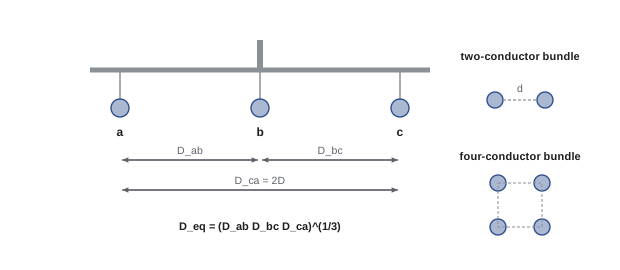
At 345 kV and above, each phase uses two to four (sometimes more) subconductors held apart by spacers, typically 0.3 to 0.5 m. Bundling increases the effective radius of the phase, which lowers inductance, raises capacitance (both increasing the power the line can carry, as shown below), and, most importantly, reduces the electric field at the conductor surface, limiting corona discharge, audible noise and radio interference. For a bundle of two subconductors at spacing \(d\), the GMR is \(\sqrt{D_s d}\), and for four, \(1.09\sqrt[4]{D_s d^3}\).

Line models

A line is described by its series impedance \(z = r + jx\) and shunt admittance \(y = jb\) per unit length. For analysis, the relationship between sending-end and receiving-end quantities is written with the two-port ABCD parameters:

with per-phase line-to-neutral voltages. For a symmetrical line, \(A = D\), and \(AD - BC = 1\). Three models are used depending on length:

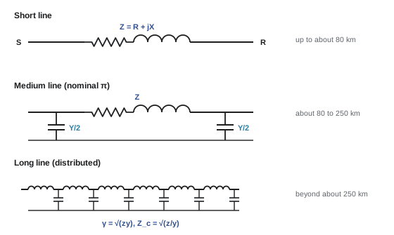
• Short line (up to about 80 km): shunt capacitance is neglected; the line is a series impedance \(Z = z\ell\), with \(A = D = 1\), \(B = Z\) and \(C = 0\).
• Medium line (about 80 to 250 km): the nominal π model places half the total shunt admittance \(Y = y\ell\) at each end, giving \(A = D = 1 + ZY/2\), \(B = Z\) and \(C = Y(1 + ZY/4)\).
• Long line (beyond about 250 km): the distributed nature must be modelled exactly, using the propagation constant \(\gamma = \sqrt{zy}\) and the characteristic impedance \(Z_c = \sqrt{z/y}\):

The exact model can also be represented by an equivalent π circuit with slightly corrected element values, which is how load flow programs model long lines.

import numpy as np

f = 60.0
r, x, b = 0.025, 0.33, 5.0e-6           # ohm/km, ohm/km, S/km (500 kV line, bundled conductors)
z, y = r + 1j * x, 1j * b
Zc = np.sqrt(z / y); gamma = np.sqrt(z * y)
V_LL = 500e3
print(f"characteristic impedance |Zc| = {abs(Zc):.0f} ohm,  SIL = {V_LL ** 2 / abs(Zc) / 1e6:.0f} MW")

def abcd_exact(L):
    gl = gamma * L
    return np.cosh(gl), Zc * np.sinh(gl), np.sinh(gl) / Zc, np.cosh(gl)

def abcd_pi(L):                          # nominal pi
    Z, Y = z * L, y * L
    return 1 + Z * Y / 2, Z, Y * (1 + Z * Y / 4), 1 + Z * Y / 2

for L in [100, 300, 600]:
    A, B, C, D = abcd_exact(L)
    Ap, Bp, Cp, Dp = abcd_pi(L)
    print(f"{L:4d} km: exact A = {A:.4f}  pi A = {Ap:.4f}   exact |B| = {abs(B):6.1f}  pi |B| = {abs(Bp):6.1f} ohm"
          f"   open-circuit Vr/Vs = {1 / abs(A):.3f}")

# receiving-end voltage for 300 km with |Vs| = 1.0 pu, unity-power-factor loads
from scipy.optimize import brentq
L = 300
A, B, C, D = abcd_exact(L)
Vs = V_LL / np.sqrt(3)
for P_MW in [0, 500, 972, 1200, 1500]:
    P1 = P_MW * 1e6 / 3                              # per phase
    g = lambda Vr: abs(A * Vr + B * P1 / Vr) - Vs    # Vr taken as the angle reference
    grid = np.linspace(1.6 * Vs, 0.2 * Vs, 400)      # search downward for the upper (normal) solution
    vals = np.array([g(v) for v in grid])
    idx = np.where(np.sign(vals[:-1]) != np.sign(vals[1:]))[0]
    if len(idx) == 0:
        print(f"P = {P_MW:4d} MW: no solution, beyond the maximum power the line can deliver")
        continue
    Vr = brentq(g, grid[idx[0] + 1], grid[idx[0]])
    delta = np.degrees(np.angle(A * Vr + B * P1 / Vr))
    print(f"P = {P_MW:4d} MW: receiving voltage = {Vr / Vs:.3f} pu, angle across line = {delta:5.1f} deg")

characteristic impedance |Zc| = 257 ohm,  SIL = 972 MW
 100 km: exact A = 0.9918+0.0006j  pi A = 0.9918+0.0006j   exact |B| =   33.0  pi |B| =   33.1 ohm   open-circuit Vr/Vs = 1.008
 300 km: exact A = 0.9267+0.0055j  pi A = 0.9257+0.0056j   exact |B| =   96.8  pi |B| =   99.3 ohm   open-circuit Vr/Vs = 1.079
 600 km: exact A = 0.7173+0.0203j  pi A = 0.7030+0.0225j   exact |B| =  179.5  pi |B| =  198.6 ohm   open-circuit Vr/Vs = 1.393
P =    0 MW: receiving voltage = 1.079 pu, angle across line =   0.3 deg
P =  500 MW: receiving voltage = 1.045 pu, angle across line =  11.0 deg
P =  972 MW: receiving voltage = 0.959 pu, angle across line =  23.4 deg
P = 1200 MW: receiving voltage = 0.865 pu, angle across line =  32.7 deg
P = 1500 MW: no solution, beyond the maximum power the line can deliver

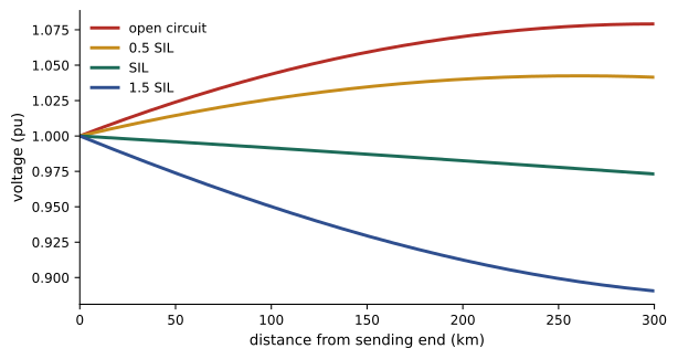
For 100 km the nominal π model is essentially exact; at 300 km it is within a few percent; at 600 km its errors exceed 10% and the exact model is needed. Unloaded, the receiving voltage of the 300 km line rises 8% above the sending voltage, and of the 600 km line 39%. Under load at unity power factor, the receiving voltage falls, reaching about 0.96 pu at the surge impedance loading of 972 MW (slightly below 1.0 because the line has resistance), and no solution exists at 1500 MW: the line simply cannot deliver that much power without voltage support.

Surge impedance loading and the Ferranti effect

If a lossless line is terminated in its characteristic impedance \(Z_c\), the reactive power generated by the shunt capacitance exactly balances the reactive power absorbed by the series inductance, and the voltage magnitude is the same all along the line. The power delivered in this condition is the surge impedance loading:

Overhead lines have characteristic impedances of about 250 to 400 Ω (lower for bundled conductors), giving SILs of roughly 40 MW at 138 kV, 140 MW at 230 kV, 400 MW at 345 kV, 950 MW at 500 kV and 2200 MW at 765 kV. Below SIL, a line generates net reactive power and voltages tend to rise; above SIL, it absorbs reactive power and voltages fall.

The extreme case is an open-circuited line. The charging current flowing through the series inductance raises the receiving voltage to \(V_R = V_S/\cos\beta\ell\) for a lossless line, where \(\beta = 2\pi/\lambda\) and the wavelength at 60 Hz is about 5000 km. This voltage rise on lightly loaded long lines is the Ferranti effect, and it is controlled with shunt reactors switched in at light load.

Power transfer and loadability

For a line modelled by its series reactance \(X\) (neglecting resistance and shunt capacitance), with sending and receiving voltages \(V_S\angle\delta\) and \(V_R\angle 0\), the real power transferred is

Real power flows from the leading to the lagging end, governed by the angle \(\delta\); it reaches a theoretical maximum \(V_SV_R/X\) at \(\delta = 90°\), the steady-state stability limit. Reactive power flows from the higher voltage magnitude to the lower, and for small angles \(Q_R \approx V_R(V_S - V_R)/X\). This decoupling, angles for real power and magnitudes for reactive power, is the foundation of the fast load flow methods in Lesson 6.

Limits on line loading

The power a line can carry is limited by different factors depending on its length:

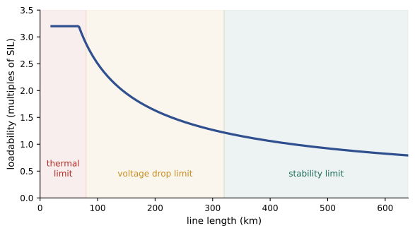
• Thermal limit: conductor temperature, which sets sag and clearance to ground, and annealing of aluminium. It governs short lines (up to about 80 km). Ratings depend on ambient temperature and wind, and dynamic line ratings that use real-time weather can safely increase capacity.
• Voltage drop limit: the receiving voltage must stay within about 5% of nominal. It governs medium lines.
• Stability limit: the angle across the line must stay well below 90°, with a margin of 30% or more. It governs long lines.

The St. Clair curve summarizes these as loadability in multiples of SIL: roughly 3 SIL at 80 km, 1.5 SIL at 300 km and about 1 SIL at 500 km for uncompensated lines.

Compensation and FACTS

Long lines are compensated to raise their capacity and control voltage:

• Series capacitors cancel part of the line reactance, commonly 30 to 70%. Since \(P_{\max} = V_SV_R/X\), 50% compensation doubles the theoretical transfer limit. Series capacitors require protection against overvoltage during faults and studies for subsynchronous resonance with nearby turbine generators.
• Shunt reactors absorb the charging reactive power at light load, controlling the Ferranti rise; shunt capacitors supply reactive power at heavy load, supporting voltage.
• Flexible AC transmission systems (FACTS) use power electronics for fast, continuous control: static var compensators and STATCOMs regulate voltage by injecting or absorbing reactive power, and thyristor-controlled series capacitors and unified power flow controllers adjust line impedance or angle to direct power flows.

Underground cables

Underground cables are used in cities, at water crossings and where overhead lines cannot be permitted. Their conductors are close together and surrounded by insulation with a relative permittivity of 2.3 to 4, so their capacitance is 20 to 50 times that of an overhead line and their characteristic impedance only 30 to 60 Ω. The charging current is large: a 230 kV cable may draw 10 to 20 A per kilometre, so beyond a few tens of kilometres the charging current alone approaches the thermal rating, leaving no capacity for load unless shunt reactors are installed along the route. This is why long cable connections, such as offshore wind farms and undersea interconnectors, use HVDC. Cables also cost five to fifteen times as much as overhead lines, take longer to repair, and have thermal ratings limited by the soil's ability to carry away heat.

Lesson 5 builds on the reactive behaviour of lines described here to study voltage control and voltage stability, and Lesson 8 uses the power-angle relation in stability analysis.