
ELE-370 · Lesson 8 of 12 · 31 min
Induction machine dynamics, control and generation
Lesson 7 analysed the induction motor in steady state on a fixed-frequency supply and introduced variable-frequency drives. In practice, engineers must also answer dynamic questions: how long a motor takes to bring a heavy load up to speed and whether it will overheat doing so, what torque a drive can deliver at low speed, how modern drives control torque as precisely as a DC machine, how motors are braked, and how the same machine works as a generator. This lesson covers starting dynamics, scalar (V/f) control and its limits, field-oriented control with the Clarke and Park transforms, braking methods, duty cycles, and induction generators including the doubly fed machines used in many wind turbines.
Starting dynamics
The speed of a motor and its load follows Newton's second law for rotation:
where \(J\) is the total moment of inertia of the motor rotor, coupling and load, referred to the motor shaft. The difference between motor and load torque, the accelerating torque, varies with speed, so the acceleration time is found by integrating:
Loads have characteristic torque-speed shapes: centrifugal fans and pumps need torque rising with the square of speed, conveyors and hoists roughly constant torque, and machine tools constant power. A load connected through a gearbox of ratio \(n\) (motor speed over load speed) has its inertia referred to the motor shaft divided by \(n^2\).
During starting, the rotor copper loss equals the air-gap power times the slip, so it is very high at low speed. For a motor accelerating an inertia with no load torque, the energy dissipated in the rotor exactly equals the kinetic energy delivered to the load; with load torque it is more. A motor driving a high-inertia load, such as a large fan, centrifuge or crusher, may take many seconds to start and heat its rotor bars severely, so manufacturers specify a maximum safe stall time and the number of starts permitted per hour.
import numpy as np

# Starting a fan direct-on-line: integrate J dw/dt = T_motor - T_load to find acceleration time and rotor heat.
R1, X1, R2, X2, Xm = 0.20, 0.80, 0.25, 0.80, 30.0          # same 50 hp, 575 V, 4-pole motor
ws = 4 * np.pi * 60 / 4                                    # 188.5 rad/s
def motor(s, V):
    Z2 = R2 / s + 1j * X2
    Zin = R1 + 1j * X1 + Z2 * 1j * Xm / (Z2 + 1j * Xm)
    I1 = V / Zin
    I2 = I1 * 1j * Xm / (Z2 + 1j * Xm)
    return 3 * abs(I2) ** 2 * R2 / s / ws, abs(I1)

def start(J, V_pu, T_load_full=160.0, dt=0.001):
    w, t, rotor_heat, peak_I = 0.0, 0.0, 0.0, 0.0
    V = 575 / np.sqrt(3) * V_pu
    while w < 0.95 * ws and t < 60:
        s = 1 - w / ws
        T, I = motor(s, V)
        T_load = T_load_full * (w / ws) ** 2              # fan torque rises with speed squared
        rotor_heat += T * ws * s * dt                      # rotor copper loss = air-gap power x slip
        peak_I = max(peak_I, I)
        w += (T - T_load) / J * dt
        t += dt
    return t, rotor_heat, peak_I, w / ws

for J, V_pu, label in ((2.0, 1.0, "small fan, full voltage"), (20.0, 1.0, "large fan wheel, full voltage"),
                       (20.0, 0.85, "large fan wheel, 85% voltage dip"), (20.0, 0.6, "large fan wheel, soft starter held at 60%")):
    t, heat, Ipk, speed = start(J, V_pu)
    ke = 0.5 * J * (0.95 * ws) ** 2
    result = f"time {t:5.2f} s" if speed >= 0.95 else f"stuck at {speed:.0%} speed after 60 s"
print(f"{label:40s}: J = {J:4.1f} kg m2, {result}, starting current {Ipk:4.0f} A, rotor heat {heat / 1000:6.1f} kJ (kinetic energy {ke / 1000:5.1f} kJ)")small fan, full voltage : J = 2.0 kg m2, time 1.58 s, starting current 202 A, rotor heat 39.1 kJ (kinetic energy 32.1 kJ) large fan wheel, full voltage : J = 20.0 kg m2, time 15.82 s, starting current 202 A, rotor heat 390.3 kJ (kinetic energy 320.7 kJ) large fan wheel, 85% voltage dip : J = 20.0 kg m2, time 23.38 s, starting current 172 A, rotor heat 408.5 kJ (kinetic energy 320.7 kJ) large fan wheel, soft starter held at 60%: J = 20.0 kg m2, stuck at 91% speed after 60 s, starting current 121 A, rotor heat 509.7 kJ (kinetic energy 320.7 kJ)
The equivalent circuit used here has a single rotor cage, which underestimates the starting torque of a real Design B motor whose deep or double-cage bars raise rotor resistance at standstill (Lesson 7), but the trends are right. Ten times the inertia means ten times the acceleration time and rotor heat. Rotor heating exceeds the kinetic energy stored, as expected with load torque. An 85% voltage dip, common when a large motor starts on a weak supply, cuts torque to 72% and lengthens the start by half. Holding a soft starter at 60% voltage leaves the motor stuck at 91% speed with high slip, dissipating heat continuously: a soft starter must ramp to full voltage, and its current limit must be set high enough for the load. Protection must allow the normal start but trip a stalled or excessively long start (Lesson 12).
Worked problem
Acceleration time with average torque
A motor with an average accelerating torque of 120 N·m over its start drives a load whose total inertia referred to the motor is 8 kg·m². How long does it take to reach 1,750 rpm?
Show solution
- \(\omega_f = 1{,}750 \times 2\pi/60 = 183.3\) rad/s.
- \(t = J\omega_f/T_{acc} = 8 \times 183.3/120 = 12.2\) s.
- Kinetic energy stored: \(\tfrac{1}{2} \times 8 \times 183.3^2 = 134\) kJ, so the rotor dissipates at least this much.
Answer: About 12 s, during which the rotor absorbs at least 134 kJ. The designer must check this against the motor's permitted starting time and the thermal limit of the rotor, and confirm that the protection will not trip during a normal start.
Scalar (V/f) control
The simplest drive control keeps the ratio of voltage to frequency constant, so that the air-gap flux stays near its rated value (Lesson 1). Because the slip speed at a given torque is roughly independent of frequency when flux is constant, the torque-speed curve simply shifts along the speed axis as frequency changes. This works well above about 10% of rated speed, but at low frequency the stator resistance drop becomes significant relative to the reduced voltage, the air-gap flux falls, and so does the available torque. Drives add a voltage boost at low frequency (IR compensation) to restore flux.
import numpy as np

# 575 V, 60 Hz, 4-pole, 50 hp (37 kW) induction motor, per-phase parameters at 60 Hz (ohms)
R1, X1, R2, X2, Xm = 0.20, 0.80, 0.25, 0.80, 30.0
V_rated, f_rated, poles = 575 / np.sqrt(3), 60, 4

def torque(s, f, V):
    k = f / f_rated                                  # reactances scale with frequency
    ws = 4 * np.pi * f / poles                       # synchronous speed, mechanical rad/s
    Z2 = R2 / s + 1j * X2 * k
    Zm = 1j * Xm * k
    Zin = R1 + 1j * X1 * k + Z2 * Zm / (Z2 + Zm)
    I1 = V / Zin
    I2 = I1 * Zm / (Z2 + Zm)
    return 3 * abs(I2) ** 2 * R2 / s / ws, abs(I1)

def breakdown(f, V):
    s = np.linspace(0.002, 1, 5000)
    T = np.array([torque(x, f, V)[0] for x in s])
    k = np.argmax(T)
    return T[k], s[k], torque(1.0, f, V)

for f in (60, 30, 10, 5):
    V = V_rated * f / f_rated                        # constant V/f
    Tmax, smax, (Tst, Ist) = breakdown(f, V)
    V_boost = V + 15 * (1 - f / f_rated)            # IR compensation: add about 15 V per phase at zero frequency
    Tmax_b, _, _ = breakdown(f, V_boost)
    print(f"{f:2d} Hz, V/f = const ({V * np.sqrt(3):5.0f} V line): breakdown torque {Tmax:6.0f} N m at slip speed {smax * 120 * f / poles:4.0f} rpm; with IR boost to {V_boost * np.sqrt(3):4.0f} V: {Tmax_b:6.0f} N m")
T_rated = 37000 / (1740 * 2 * np.pi / 60)
print(f"rated torque {T_rated:.0f} N m")60 Hz, V/f = const ( 575 V line): breakdown torque 467 N m at slip speed 283 rpm; with IR boost to 575 V: 467 N m 30 Hz, V/f = const ( 288 V line): breakdown torque 414 N m at slip speed 276 rpm; with IR boost to 300 V: 452 N m 10 Hz, V/f = const ( 96 V line): breakdown torque 266 N m at slip speed 227 rpm; with IR boost to 117 V: 400 N m 5 Hz, V/f = const ( 48 V line): breakdown torque 161 N m at slip speed 150 rpm; with IR boost to 72 V: 361 N m rated torque 203 N m
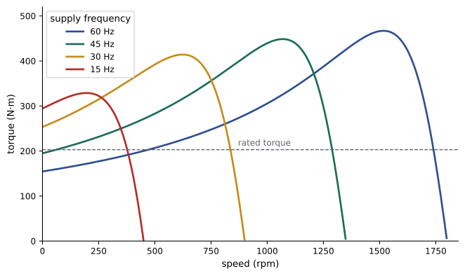
At 60 Hz the motor's breakdown torque is about 2.3 times rated. Under pure V/f it falls to 1.3 times rated at 10 Hz and below rated at 5 Hz, so the motor could stall when starting a heavily loaded conveyor. A modest boost restores most of it. Too much boost over-fluxes the motor at light load, raising magnetizing current and heating, which is why drives offer automatic boost based on measured current. V/f control with slip compensation (raising frequency slightly as load increases) gives speed regulation of about 1% and suits fans, pumps and conveyors, which are the majority of drive applications. It does not control torque directly and responds slowly to load changes.
Field-oriented (vector) control
A separately excited DC motor (Lesson 5) is easy to control because flux and torque are set by separate currents: field current sets flux, and armature current, at 90° to the flux, sets torque. Field-oriented control (FOC) gives an AC motor the same property by describing the stator currents in a reference frame that rotates with the rotor flux. In that frame, the current splits into two components that appear as DC quantities in steady state:
- The d-axis (direct) current \(i_d\), aligned with the rotor flux, which sets the flux like a field current.
- The q-axis (quadrature) current \(i_q\), at 90° to the flux, which produces torque like an armature current.
Two transforms get there. The Clarke transform converts the three phase currents into two orthogonal components \(i_\alpha\) and \(i_\beta\) in a stationary frame, and the Park transform rotates them by the flux angle \(\theta\) to give \(i_d\) and \(i_q\):
import numpy as np

# Clarke and Park transforms: balanced three-phase currents become constant d and q currents
# in a reference frame rotating with the rotor flux.
f, I_pk = 40.0, 60.0
w = 2 * np.pi * f
phi = np.radians(-50)                       # current leads the flux axis by 50 deg: d = flux, q = torque

def clarke(ia, ib, ic):                     # amplitude-invariant form
    alpha = (2 * ia - ib - ic) / 3
    beta = (ib - ic) / np.sqrt(3)
    return alpha, beta

def park(alpha, beta, theta):
    d = alpha * np.cos(theta) + beta * np.sin(theta)
    q = -alpha * np.sin(theta) + beta * np.cos(theta)
    return d, q

print("  t (ms)     ia      ib      ic   |  alpha    beta  |    id      iq")
for ms in (0.0, 2.5, 5.0, 7.5, 10.0):
    t = ms / 1000
    ia = I_pk * np.cos(w * t - phi)
    ib = I_pk * np.cos(w * t - phi - 2 * np.pi / 3)
    ic = I_pk * np.cos(w * t - phi + 2 * np.pi / 3)
    a, b = clarke(ia, ib, ic)
    d, q = park(a, b, w * t)                # frame angle follows the flux, which rotates at w
    print(f"{ms:7.1f} {ia:7.1f} {ib:7.1f} {ic:7.1f}   | {a:6.1f} {b:7.1f}  | {d:6.1f} {q:7.1f}")
# A step in torque command: only iq changes; the flux current id is held
print(f"flux current id = {I_pk * np.cos(phi):.1f} A sets the rotor flux; torque is proportional to flux x iq = {I_pk * np.sin(-phi):.1f} A") t (ms) ia ib ic | alpha beta | id iq
0.0 38.6 20.5 -59.1 | 38.6 46.0 | 38.6 46.0
2.5 4.2 49.7 -53.9 | 4.2 59.9 | 38.6 46.0
5.0 -31.8 60.0 -28.2 | -31.8 50.9 | 38.6 46.0
7.5 -55.6 47.3 8.4 | -55.6 22.5 | 38.6 46.0
10.0 -58.2 16.5 41.7 | -58.2 -14.5 | 38.6 46.0
flux current id = 38.6 A sets the rotor flux; torque is proportional to flux x iq = 46.0 AThe phase currents and the stationary \(\alpha\)-\(\beta\) components vary sinusoidally, but in the frame rotating with the flux, \(i_d\) and \(i_q\) are constant. A drive therefore regulates two DC quantities with ordinary PI controllers, then transforms the voltage commands back to three phases for the PWM inverter. The electromagnetic torque is
proportional to rotor flux \(\lambda_r\) and \(i_q\), just as DC machine torque is proportional to flux and armature current. A step change in torque command changes \(i_q\) within a few milliseconds while the flux, which changes slowly, is held constant. The difficulty is knowing the flux angle. In indirect FOC, the drive computes it by adding the rotor position, from an encoder, to the integral of the slip frequency given by \(\omega_{slip} = i_q/(\tau_r i_d)\), where \(\tau_r = L_r/R_r\) is the rotor time constant. Errors in the rotor time constant, which changes as the rotor heats, degrade performance, so drives estimate it online. Sensorless vector control estimates speed and flux from measured voltages and currents, avoiding the encoder, and works well except near zero speed.
Direct torque control (DTC) is an alternative that estimates stator flux and torque every few tens of microseconds and selects inverter switching states directly from a table to keep them within hysteresis bands. It responds even faster than FOC and needs no current regulators or modulator, at the cost of variable switching frequency and more torque ripple.
| Method | Speed accuracy | Torque response | Low-speed torque | Typical applications |
|---|---|---|---|---|
| V/f (open loop) | 1 to 3% | slow, not controlled | limited below about 5 Hz | fans, pumps, simple conveyors |
| Sensorless vector | 0.1 to 0.5% | about 10 ms | good to about 1 Hz | mixers, extruders, general industry |
| Vector with encoder | 0.01% | 1 to 5 ms | full torque at zero speed | hoists, cranes, winders, machine tools |
| Direct torque control | 0.1 to 0.5% (sensorless) | under 5 ms | good | high-dynamic industrial drives |
Braking and four-quadrant operation
A drive operates in four quadrants of the torque-speed plane: motoring forward, braking forward, motoring in reverse, and braking in reverse. Braking means the machine acts as a generator, converting kinetic or potential energy into electrical energy, which must go somewhere:
- Dynamic (resistor) braking: with a standard diode rectifier, regenerated energy raises the DC bus voltage; a brake chopper switches it into a resistor, which turns it into heat.
- Regenerative braking: an active front end (a second inverter on the supply side) or a regenerative unit returns energy to the supply. It suits frequent braking with large energy, such as cranes, elevators, downhill conveyors and test stands.
- DC injection braking: DC current in the stator creates a stationary field, and the rotor dissipates its kinetic energy as heat; it is cheap but slow and heats the motor.
- Plugging: reversing two phases at speed brakes fiercely, but dissipates three times the kinetic energy in the rotor; it is rarely acceptable for large motors.
- Mechanical brakes hold loads at standstill and act in emergencies; a hoist must never rely on electrical braking alone to hold a load.
Duty cycles and thermal rating
A motor's rating depends on how it is used. IEC 60034-1 defines duty types: S1 continuous running at constant load; S2 short-time duty; S3 intermittent periodic duty (for example, 40% on in each 10-minute cycle); S4 and S5 intermittent with starting and braking; S6 continuous operation with intermittent load; and S9 non-periodic load and speed variations typical of drive applications. A motor with a short duty can be smaller than its peak power suggests, because its thermal time constant, typically tens of minutes for medium motors, smooths the heating. For a cyclic load, the RMS torque over the cycle is a useful first check of thermal adequacy:
Self-cooled motors on drives also lose cooling at low speed, because their shaft-mounted fan slows: a standard motor may need derating to 50 to 80% torque at 10 to 20% speed, while inverter-duty motors with separate blowers deliver full torque at any speed.
Induction generators
Driven above synchronous speed, an induction machine has negative slip and delivers power to the supply. Grid-connected squirrel-cage induction generators are simple and robust and were used in early fixed-speed wind turbines and in small hydro plants. They must draw reactive power from the grid or from capacitors to magnetize, and their output frequency is fixed by the grid. A stand-alone induction generator can self-excite with capacitors across its terminals if the rotor has residual magnetism, but its voltage and frequency vary with load and speed.
Most large wind turbines built from the late 1990s to the 2010s use doubly fed induction generators (DFIG). The stator connects directly to the grid, and the wound rotor connects through slip rings to a back-to-back converter that injects rotor currents at slip frequency. The converter controls the rotor current in a rotating frame, as in FOC, so the generator can operate over about ±30% around synchronous speed with independent control of active and reactive power. Because the rotor carries only the slip power, the converter needs to be rated at only about 30% of the generator rating, which made DFIGs economical; turbines with full-scale converters and permanent magnet or synchronous generators (Lesson 11) are now increasingly common, especially offshore.
At 20% above synchronous speed (\(s = -0.2\)), a DFIG delivers 120% of its stator power to the grid, with the extra 20% flowing out of the rotor through the converter. Grid codes, including those of Canadian utilities and system operators, require wind generators to ride through voltage dips and support voltage with reactive current, which DFIGs achieve with converter controls and a crowbar or chopper to protect the converter during faults.
Common mistakes
MistakeChecking only that starting torque exceeds load torque at standstill.
InsteadCheck accelerating torque over the whole speed range, starting time and rotor heating.
MistakeLeaving a soft starter at reduced voltage for a high-torque load.
InsteadRamp to full voltage and set current limits to suit the load.
MistakeUsing V/f control for a hoist needing full torque at zero speed.
InsteadUse vector control with an encoder and a mechanical brake.
MistakeRunning a standard TEFC motor at full torque at low speed for long periods.
InsteadDerate for reduced fan cooling or use an inverter-duty motor with a separate blower.
MistakeRelying on electrical braking to hold a suspended load.
InsteadUse a mechanical holding brake.
Summary and key terms
- Acceleration follows \(J\, d\omega/dt = T_{motor} - T_{load}\); high inertia lengthens starts and heats the rotor.
- Constant V/f keeps flux constant and shifts torque-speed curves; IR boost restores low-speed torque.
- Field-oriented control uses Clarke and Park transforms to control flux (\(i_d\)) and torque (\(i_q\)) separately, like a DC machine.
- DTC selects inverter states directly from estimated flux and torque for very fast response.
- Braking uses resistors, regeneration, DC injection or mechanical brakes; regenerated energy must be absorbed.
- Duty cycles and RMS torque determine thermal rating; self-cooled motors need derating at low speed.
- Induction generators run at negative slip; DFIGs control rotor current through a converter rated at about 30%.
- Accelerating torque
- The difference between motor torque and load torque.
- Moment of inertia
- Resistance of a rotating body to changes in speed.
- IR compensation
- Voltage boost at low frequency to offset stator resistance drop.
- Field-oriented control
- Control of flux and torque currents in a frame rotating with the rotor flux.
- Clarke transform
- Conversion of three-phase quantities to two orthogonal stationary components.
- Park transform
- Rotation of stationary components into a rotating reference frame.
- Rotor time constant
- The ratio \(L_r/R_r\) governing rotor flux dynamics.
- Regenerative braking
- Braking that returns energy to the supply.
- Duty type
- A standard pattern of load and operation for motor rating.
- Doubly fed induction generator
- A wound-rotor generator with a converter controlling rotor currents.
Practice problems
Work each problem on paper first, then reveal the answer to check.
Time to accelerate 5 kg·m² to 1,780 rpm with 80 N·m average accelerating torque?
Show answer
\(5 \times 186.4/80 = 11.7\) s.
A 100 kg·m² load runs through a 10:1 gearbox. Inertia referred to the motor?
Show answer
1 kg·m².
Minimum rotor heat when accelerating 10 kg·m² to 188 rad/s with no load torque?
Show answer
\(\tfrac{1}{2} \times 10 \times 188^2 = 177\) kJ.
Why does V/f torque fall at low frequency?
Show answer
Stator resistance drop reduces air-gap flux.
Which current sets torque in FOC?
Show answer
The q-axis current.
What does the Park transform need?
Show answer
The angle of the rotor flux (reference frame).
RMS torque of 300 N·m for 10 s and 100 N·m for 50 s?
Show answer
\(\sqrt{(900{,}000 + 500{,}000)/60} = 153\) N·m.
Name two ways to handle regenerated energy in a drive.
Show answer
Brake chopper and resistor; active front end.
Grid power of a DFIG with 2 MW stator power at s = −0.15?
Show answer
2.3 MW.
Why must an induction generator draw reactive power?
Show answer
To magnetize the machine.
Lesson quiz · 5 questions
Score 60% or more to complete this lesson.
Create a free account to save your progress, take quizzes and earn a certificate.