
BAS-130 · Lesson 12 of 12 · 27 min
Putting it together: a discharge air temperature loop
▶ Video coming soon A video version of this lesson is on the way.
On Thursday, October 29, Gus Thibodeaux forwarded Quillon a complaint from the Tilden lecture wing. Instructors in the two large halls said the air from the ceiling diffusers felt alternately warm and cool every minute or two, and one had moved her lectern away from a diffuser because of the draft. The halls are served by AHU-2, the old air handler due for replacement in 2027, whose pneumatic dampers Callie had serviced on October 8 and whose freezestat she had rewired the day before that. Prakash suggested she lead the investigation, with him watching. "You've got eleven Fridays of theory," he said. "Let's see it work." This lesson follows the job from complaint to verified fix, pulling together everything in the course.
AHU-2's discharge air temperature loop is the inner loop of a cascade, as lesson 7 described. The outer loop compares the lecture hall temperature with its setpoint and calculates a discharge air setpoint between limits. The inner loop holds the discharge air, measured just downstream of the heating coil, at that setpoint by modulating the hot water heating valve, with the economizer dampers controlled by their own mixed air loop. The complaint described exactly what a hunting inner loop would deliver to the room: air swinging warmer and cooler on a short cycle.
Step 1: read the trend
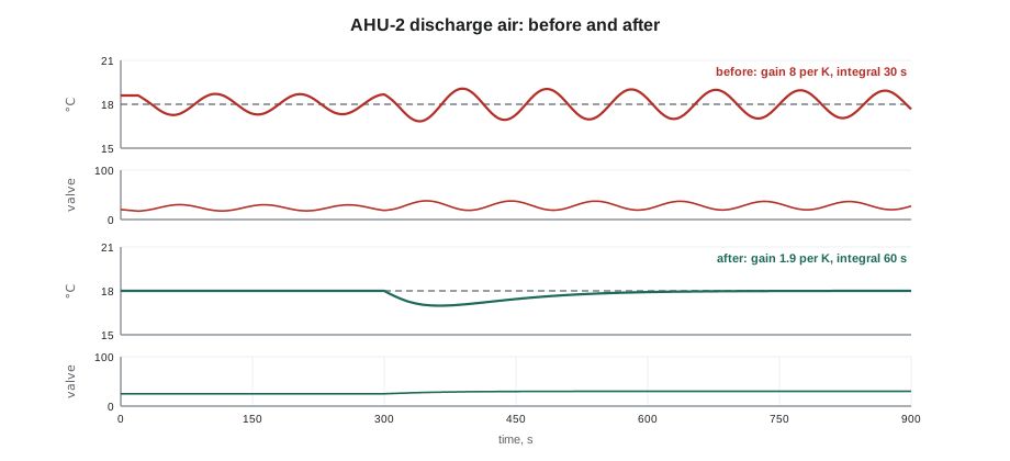
Callie began where Prakash had taught her to begin, with a trend of the setpoint, process variable and output on one graph, at a 5-second sample interval. The trend was clear. The discharge air setpoint from the outer loop was steady at about 18 °C, moving only slowly. The discharge air itself swung between about 17 and 19 °C, with a period of about a minute and a half. The heating valve output swung between about 20 and 40 in 100 on every cycle, reversing direction twice a minute. The swing had been present, at about the same size, every occupied day since mid-September.
Worked problem
What the trend says
The discharge air swings from 17 to 19 °C around an 18 °C setpoint, with a period of about 96 seconds. What are the amplitude and the frequency of the swing in cycles per hour?
Show solution
- Total swing: 19 − 17 = 2 K, so the amplitude is about 1 K either side.
- Frequency: 3,600 ÷ 96 = 37.5, about 38 cycles per hour.
Answer: An amplitude of about 1 K and about 38 cycles an hour, enough for occupants near a diffuser to feel the air change.
Callie added a wear count of her own: about 38 cycles an hour is 75 reversals of the valve's direction every hour, or 900 in a twelve-hour occupied day, far more movement than an actuator rated for normal modulating duty is designed for. Hunting is a maintenance problem as well as a comfort one.
Step 2: check the setpoint and the outer loop
In a cascade, the first question is whether the inner loop is hunting by itself or being pushed by the outer loop. If the outer loop were swinging, it would swing the inner loop's setpoint. The trend showed the opposite: a steady setpoint and a swinging process variable. Callie also checked that the outer loop's limits were sensible, 13 to 30 °C as lesson 7 described, and that the lecture hall sensors were reading correctly against a portable thermometer. The outer loop was not the problem.
Step 3: the manual test
Lesson 10's first test was next. With Gus's agreement and the hall empty between lectures, Callie put the heating valve output in manual at 35 in 100, close to its average on the trend, and watched for ten minutes. The discharge air settled at about 18.4 °C and drifted only slowly as the mixed air temperature changed. The swing stopped. Whatever was causing it was inside the loop: its settings, its final element, its sensor or its signal. She returned the loop to automatic and noted the time on the work order.
Step 4: the final element
Before touching any settings, Callie checked the heating valve and its actuator. The valve had been fitted with an electric actuator in 2012. She stroked it in manual in steps of 10 in 100, watching the position indicator and the coil's leaving water temperature, and it followed every step without sticking or lag. The coupling was tight and marked with a witness line. The mixed air dampers were pneumatic, and lesson 11's visit had found the return damper without a positioner, lagging its command; but the mixed air loop was steady on the trend, and its small hysteresis showed up only as a slow drift, not a two-minute swing. The valve also looked reasonably sized: at the coldest point of the morning trend it reached about 80 in 100, so its travel was well used.
Step 5: the sensor
The discharge air sensor was a single-point probe mounted about 0.6 m downstream of the heating coil, in a short section of casing before the supply fan. Callie held a portable probe at several points across the casing with the coil heating and found readings that varied by more than 3 K from side to side: the air leaving the coil was stratified, warmer near the supply header and cooler near the return. The fixed probe was sitting in a stream whose temperature shifted as the valve moved and the coil's warm zone grew and shrank. That made the loop see exaggerated swings and react to them.
There were two choices. An averaging sensor across the coil face would read the true average temperature, as BAS-120 explained, and would be the better long-term fix. Moving the existing probe downstream of the supply fan, where the fan mixes the air thoroughly, would cure the stratification immediately, at the cost of a little transport delay. With the unit being replaced in 2027, Prakash suggested moving the probe now and ordering an averaging sensor only if the move did not do enough.
Worked problem
Delay added by moving the sensor
The new location is 3 m further along the airstream, where the air moves at about 3 m/s. How much transport delay does the move add?
Show solution
- Delay = 3 ÷ 3 = 1 s.
Answer: About one second, negligible compared with the loop's own dead time, in exchange for a reading of well-mixed air.
Step 6: the settings and their history
Only now did Callie open the loop's settings. The gain was 8 per K, with an integral time of 30 seconds. The controller's change log, and a comment field Sophie had insisted on years earlier, showed that in mid-September someone had raised the gain from 2 and shortened the integral time from 90 seconds, with the comment "faster warm-up". The change coincided exactly with the start of the swing on the trend. It had been made in good faith, to speed up morning warm-up, but it had made the loop far too aggressive for a process with a stratified sensor. Callie recorded the existing settings on the work order before changing anything.
| Setting | Before September | After September change | Effect |
|---|---|---|---|
| Gain | 2 per K | 8 per K | Four times more aggressive |
| Throttling range | 50 K | 12.5 K | Much narrower |
| Integral time | 90 s | 30 s | Three times faster integral |
Step 7: a step test and new settings
On Friday, October 30, Callie and Prakash arrived at 7:00, before the halls were occupied, moved the sensor to its new position, and ran a step test with the loop in manual. With the discharge air steady, Callie stepped the heating valve from 30 to 40 in 100 and recorded the response.
Worked problem
Reading the AHU-2 step test
After the valve step from 30 to 40 in 100, nothing changed for about 20 seconds; the discharge air then rose and settled 4.0 K higher, reaching 63 in 100 of that change 80 seconds after the step. Find the process gain, dead time and time constant, then the lambda PI settings with lambda equal to the time constant.
Show solution
- Process gain: 4.0 ÷ 10 = 0.4 K per unit of output.
- Dead time: 20 s. Time constant: 80 − 20 = 60 s.
- Gain: Kc = 60 ÷ (0.4 × (60 + 20)) = 60 ÷ 32 = 1.875, about 1.9 per K.
- Throttling range: 100 ÷ 1.875 = about 53 K. Integral time: 60 s.
Answer: A gain of about 1.9 per K with an integral time of 60 seconds, close to the loop's original settings and far gentler than the September change.
The ratio of dead time to time constant, 20 to 60, was a third, higher than the converter's quarter in lesson 6. That alone argued for gentle settings. Prakash also pointed out what the step test could not show: the stratified sensor had made the process look jumpier than it was, so the September change had been even worse than it seemed on paper.
Step 8: check the result
Callie entered the new settings and put the loop back in automatic. She tested it two ways, as lesson 6 described. First, she raised the discharge air setpoint by 2 K with the outer loop's output held in manual. The discharge air rose smoothly to the new setpoint in about three minutes, overshooting by about 0.3 K, and settled. Second, she let the mixed air loop change the outdoor air damper as the morning warmed, a real load disturbance. The discharge air dipped by about 0.4 K and recovered in about two minutes without swinging. Then she returned the outer loop to automatic and watched the system through the first lecture at 8:30.
She also checked the things around the loop that the course had covered. The heating loop was disabled with its output held at zero when the supply fan was off, so it could not wind up overnight, as lesson 5 warned. The start sequence released the loop 30 seconds after fan proof, as lesson 9 described. And the cascade's outer loop stopped integrating when the discharge air setpoint reached its limits. All three were in order.
Worked problem
Comparing before and after
Before the work, the discharge air swung about ±1 K at about 38 cycles an hour. On Monday, November 2, the trend from the weekend and Monday morning showed the discharge air within ±0.2 K of setpoint, with no regular cycle. By what factor did the amplitude fall?
Show solution
- 1 ÷ 0.2 = 5.
Answer: The swing was about five times smaller and no longer regular, which is the difference between a hunting loop and a healthy one following its load.
Callie looked at the Monday trend on the Tilden front end while she was in the building replacing AHU-1's mixed air sensor. Gus forwarded a one-line note from the instructor who had moved her lectern: the draft had gone.
Step 9: record and hand over
The job was not finished until it was recorded. Callie's work order listed the complaint, the trend findings, each test and its result, the old and new settings, the sensor's old and new locations, and the step test numbers. She entered the new settings and a short explanation in the controller's comment field, so that the next person tempted to speed up warm-up would see why the gain was what it was. She also added two items to the AHU-2 replacement file for Declan: an averaging discharge air sensor and a positioner, or better an electronic actuator, on the return damper. Both are plans for the new unit rather than work done now.
Prakash's last point was about warm-up itself. The September change had been made because someone wanted the halls warmer sooner on cold mornings. That was a reasonable goal, met the wrong way. A loop's settings are not the tool for start-up speed. An earlier start time, a warm-up mode that runs the outer loop with a higher discharge air limit, or the feedforward described in lesson 7 would all do it without making the loop hunt for the rest of the day. Gus agreed to look at the start schedule with Nell before the coldest weather arrived.
The method in one table
Looking back, Callie realized that the order of the steps had mattered as much as the steps themselves. Settings were the sixth thing she looked at, not the first, and by then she knew the loop's other parts were sound. Prakash's version of the same lesson, written on the back of the work order, was the table below.
| Step | Question | Tool |
|---|---|---|
| 1 | What is the loop doing? | Trend setpoint, process variable and output together |
| 2 | Is the setpoint right and steady? | Check the effective setpoint and any outer loop |
| 3 | Is the loop the source? | Hold the output in manual and watch |
| 4 | Does the final element follow its command? | Stroke it in small steps; check couplings and positioners |
| 5 | Is the sensor telling the truth? | Compare with a reference; check location, stratification and noise |
| 6 | What are the settings and who changed them? | Read and record settings and the change log |
| 7 | What does the process need? | Step test and a tuning rule |
| 8 | Does it work now? | Setpoint step, load disturbance and a day of trends |
| 9 | Will the next person understand? | Work order, comments in the program, notes for the future |
Common mistakes
MistakeStarting with the settings.
InsteadCheck the trend, setpoint, outer loop, final element and sensor first.
MistakeUsing loop gain to speed up morning warm-up.
InsteadUse the start schedule, a warm-up mode or feedforward instead.
MistakeMoving a sensor far downstream without thinking about delay.
InsteadWork out the transport delay; a short move to well-mixed air is usually worth it.
MistakeTesting a retuned loop only with a setpoint change.
InsteadAlso test a real load disturbance and watch a full day of trends.
MistakeLeaving no explanation for the new settings.
InsteadRecord them on the work order and in the controller's comments.
Summary and key terms
- A hunting inner loop in a cascade showed as a steady setpoint and a swinging process variable and output.
- The manual test proved the loop itself was the source.
- The final element was sound; the sensor was in stratified air and the settings had been made far too aggressive in September.
- Moving the sensor to well-mixed air added only about a second of delay.
- A step test and lambda tuning gave settings close to the original, gentle ones.
- The result was checked with a setpoint step, a load disturbance and a day of trends, and anti-windup, start-up and cascade limits were confirmed.
- The work was recorded, and future improvements were passed to the replacement project.
- Discharge air temperature
- The temperature of the air leaving an air handler's coils or fan.
- Stratification
- Layers or streams of air at different temperatures that have not yet mixed.
- Change log
- A controller's record of who changed which settings and when.
- Warm-up mode
- A start-up sequence that heats a building quickly before normal control begins.
- Load disturbance test
- Checking a loop's response to a real change in load rather than a setpoint change.
Practice problems
Work each problem on paper first, then reveal the answer to check.
Why did Callie check the outer loop before the inner loop's settings?
Show answer
A swinging outer loop would push the inner loop's setpoint; the trend showed a steady setpoint, so the inner loop was the source.
What did the manual test show?
Show answer
The swing stopped with the valve output held, so the cause was inside the loop.
Why move the sensor downstream of the supply fan?
Show answer
The fan mixes the air, curing the stratification, and the added delay was only about a second.
A step of 10 in 100 gives 3 K, with a 15 s dead time and a 45 s time constant. With λ = τ, what is the lambda gain?
Show answer
45 ÷ (0.3 × 60) = 2.5 per K; integral time 45 s.
Name two better ways than a higher loop gain to speed up morning warm-up.
Show answer
An earlier start, a warm-up mode or feedforward at start-up.
Lesson quiz · 5 questions
Score 60% or more to complete this lesson.
Create a free account to save your progress, take quizzes and earn a certificate.