
AI-330 · Lesson 9 of 12 · 29 min
Policy gradients and actor-critic methods
The methods so far learn values and derive a policy from them by acting greedily. Policy gradient methods take the direct route: they parameterize the policy itself, \(\pi(a \mid s, \boldsymbol\theta)\), and adjust \(\boldsymbol\theta\) by gradient ascent on the expected return. This handles continuous actions naturally (the policy can output the mean and spread of a Gaussian), can learn stochastic policies when they are optimal, and changes the policy smoothly rather than switching abruptly when one action's value overtakes another's. Actor-critic methods combine the two families, learning a policy (the actor) guided by a learned value function (the critic). They are the basis of the algorithms used for robotics, continuous control and the fine-tuning of large language models. This lesson develops the policy gradient theorem, REINFORCE, baselines, actor-critic methods, trust-region and PPO methods, continuous control algorithms, and RL from human feedback.
Parameterized policies
For discrete actions, a common choice is a softmax over action preferences \(h(s, a, \boldsymbol\theta)\), which may be linear in features or the output of a neural network:
For continuous actions, the policy can be a Gaussian whose mean \(\mu(s, \boldsymbol\theta)\) and standard deviation \(\sigma(s, \boldsymbol\theta)\) are computed by a network, with actions sampled from \(\mathcal N(\mu, \sigma^2)\). The objective is the expected return from the start state, \(J(\boldsymbol\theta) = v_{\pi_{\boldsymbol\theta}}(s_0)\), and the method performs gradient ascent \(\boldsymbol\theta \leftarrow \boldsymbol\theta + \alpha\nabla J(\boldsymbol\theta)\).
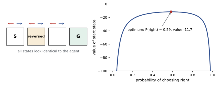
Stochastic policies can be genuinely better than any deterministic one when the agent cannot distinguish states. In a short corridor where the actions are reversed in one state but all states look the same to the agent, any deterministic policy gets stuck forever, while choosing "right" with probability about 0.59 reaches the goal in about 11.7 steps on average. Value-based methods with ε-greedy policies cannot represent this optimum; policy gradient methods find it.
The policy gradient theorem
The difficulty is that \(J\) depends on the policy both through the actions chosen and through the distribution of states visited, which depends on the unknown environment. The policy gradient theorem shows that the gradient nonetheless has a simple form that does not involve the derivative of the state distribution:
The second form follows from \(\nabla\pi = \pi\nabla\ln\pi\) (the log-derivative trick, also used in the score-function estimator of AI-320) and replacing \(q_\pi\) by the sampled return. It says: increase the log-probability of each action taken in proportion to the return that followed it. Actions followed by high returns become more likely, actions followed by low returns less likely.
For a softmax policy with linear preferences \(h = \boldsymbol\theta^\top\mathbf x(s, a)\), the gradient of the log-probability is \(\nabla\ln\pi(a \mid s) = \mathbf x(s, a) - \sum_b \pi(b \mid s)\mathbf x(s, b)\): the feature vector of the chosen action minus the policy's average feature vector.
REINFORCE
REINFORCE, introduced by Ronald Williams in 1992, is the direct Monte Carlo implementation: run an episode, then for each step update
REINFORCE is unbiased, but its gradient estimates have very high variance, because returns vary greatly from episode to episode, so it learns slowly and needs small step sizes.
Baselines
Subtracting a baseline \(b(s)\) that does not depend on the action leaves the expected gradient unchanged, because \(\sum_a b(s)\nabla\pi(a \mid s) = b(s)\nabla\sum_a\pi(a \mid s) = b(s)\nabla 1 = 0\), but can greatly reduce its variance:
A natural baseline is a learned estimate of the state value \(\hat v(S_t, \mathbf w)\), so the update increases the probability of actions that did better than expected and decreases it for actions that did worse. The quantity \(G_t - \hat v(S_t)\) estimates the advantage of the action taken.
import numpy as np

# Short corridor: states 0, 1, 2 then goal; reward -1 per step. In state 1 the actions are reversed.
# All states look identical to the agent, so the best it can do is a stochastic policy.
def env_step(s, right):
    move = 1 if right else -1
    if s == 1: move = -move
    return max(s + move, 0)

def true_value(p):                              # exact value of the start state for p = P(right)
    A = np.array([[1 - (1 - p), -p, 0], [-p, 1, -(1 - p)], [0, -(1 - p), 1]])
    A[0, 0] = p                                  # from state 0: left stays in 0, right goes to 1
    return np.linalg.solve(A, -np.ones(3))[0]

ps = np.linspace(0.05, 0.95, 181)
best = ps[np.argmax([true_value(p) for p in ps])]
print(f"optimal P(right) = {best:.2f}, value = {true_value(best):.2f}")

def reinforce(alpha, baseline, episodes=1000, seed=0):
    rng = np.random.default_rng(seed)
    theta = np.array([np.log(0.05), np.log(0.95)])   # preferences (right, left): start at P(right) = 0.05
    v = 0.0; returns = []
    for _ in range(episodes):
        s, traj = 0, []
        while s < 3 and len(traj) < 1000:
            pr = np.exp(theta[0]) / np.exp(theta).sum()
            right = rng.random() < pr
            traj.append((right, pr)); s = env_step(s, right)
        G_total = -len(traj); returns.append(G_total)
        for t, (right, pr) in enumerate(traj):
            G = -(len(traj) - t)                       # return from step t
            adv = G - (v if baseline else 0.0)
            grad = np.array([1 - pr, -(1 - pr)]) if right else np.array([-pr, pr])
            theta += alpha * adv * grad
            if baseline:
                v += 0.1 * (G - v)
    pr = np.exp(theta[0]) / np.exp(theta).sum()
    return np.mean(returns[:200]), np.mean(returns[-100:]), pr

for alpha, base in [(2 ** -12, False), (2 ** -9, False), (2 ** -9, True)]:
    res = np.array([reinforce(alpha, base, episodes=600, seed=k) for k in range(20)])
    tag = "yes" if base else "no "
    print(f"alpha = 2^{int(np.log2(alpha)):3d}, baseline {tag}: mean return, episodes 1-200: {res[:, 0].mean():7.2f};"
f" last 100: {res[:, 1].mean():6.2f}; final P(right) {res[:, 2].mean():.2f} (spread across runs {res[:, 2].std():.2f})")optimal P(right) = 0.58, value = -11.66 alpha = 2^-12, baseline no : mean return, episodes 1-200: -27.69; last 100: -12.12; final P(right) 0.49 (spread across runs 0.04) alpha = 2^ -9, baseline no : mean return, episodes 1-200: -15.81; last 100: -12.59; final P(right) 0.57 (spread across runs 0.09) alpha = 2^ -9, baseline yes: mean return, episodes 1-200: -24.19; last 100: -11.58; final P(right) 0.58 (spread across runs 0.07)
The optimal stochastic policy chooses right with probability 0.58 to 0.59, for an expected return of −11.66. With a very small step size, REINFORCE without a baseline is still far from the optimum after 600 episodes. With a larger step it learns quickly at first but its final policy is noisy, varying more between runs. With the learned baseline at the same step size, it settles closest to the optimal policy with the best final return. The baseline starts at zero and must first learn the scale of the returns, which slows the very first episodes here; in larger problems the variance reduction is usually decisive.
Actor-critic methods
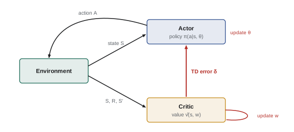
REINFORCE with a baseline still waits for complete returns. Actor-critic methods replace the return with a bootstrapped estimate, using the TD error as the advantage signal:
The critic learns state values by TD; the actor adjusts the policy in the direction the critic's TD error suggests. Bootstrapping introduces some bias but greatly reduces variance and allows learning online, step by step, in continuing tasks. Using \(n\)-step returns or generalized advantage estimation (GAE), an exponentially weighted average of \(n\)-step advantage estimates controlled by a parameter \(\lambda\) like TD(λ), tunes the bias-variance trade-off. Advantage actor-critic (A2C) and its asynchronous version (A3C) run many environment copies in parallel to collect diverse experience for each update.
Trust regions and PPO
Policy gradient steps that are too large can collapse performance: a change in parameters can change the policy, and therefore the data it will generate, dramatically. Trust region policy optimization (TRPO) limits each update so that the new policy stays within a set KL divergence of the old one. Proximal policy optimization (PPO), introduced in 2017, achieves a similar effect much more simply. It collects a batch of experience with the current policy, then takes several epochs of mini-batch gradient steps on a clipped surrogate objective:
The probability ratio \(r_t\) measures how much the new policy changes the probability of the action taken. Clipping removes the incentive to move the ratio outside \([1 - \varepsilon, 1 + \varepsilon]\), typically with \(\varepsilon = 0.2\), so that the policy improves without straying far from the policy that collected the data.
import numpy as np

# PPO clipped surrogate for one sample: L = min(ratio * A, clip(ratio, 1 - eps, 1 + eps) * A)
eps = 0.2
ratios = np.array([0.5, 0.8, 0.9, 1.0, 1.1, 1.2, 1.5, 2.0])
for A in (+1.0, -1.0):
    unclipped = ratios * A
    clipped = np.minimum(unclipped, np.clip(ratios, 1 - eps, 1 + eps) * A)
    grad_zero = np.isclose(clipped, np.clip(ratios, 1 - eps, 1 + eps) * A) & ~np.isclose(clipped, unclipped)
    print(f"advantage {A:+.0f}:")
    for r, u, c, g in zip(ratios, unclipped, clipped, grad_zero):
        note = "  (clipped: no gradient)" if g else ""
print(f" ratio {r:3.1f}: unclipped {u:+.2f} PPO objective {c:+.2f}{note}")advantage +1: ratio 0.5: unclipped +0.50 PPO objective +0.50 ratio 0.8: unclipped +0.80 PPO objective +0.80 ratio 0.9: unclipped +0.90 PPO objective +0.90 ratio 1.0: unclipped +1.00 PPO objective +1.00 ratio 1.1: unclipped +1.10 PPO objective +1.10 ratio 1.2: unclipped +1.20 PPO objective +1.20 ratio 1.5: unclipped +1.50 PPO objective +1.20 (clipped: no gradient) ratio 2.0: unclipped +2.00 PPO objective +1.20 (clipped: no gradient) advantage -1: ratio 0.5: unclipped -0.50 PPO objective -0.80 (clipped: no gradient) ratio 0.8: unclipped -0.80 PPO objective -0.80 ratio 0.9: unclipped -0.90 PPO objective -0.90 ratio 1.0: unclipped -1.00 PPO objective -1.00 ratio 1.1: unclipped -1.10 PPO objective -1.10 ratio 1.2: unclipped -1.20 PPO objective -1.20 ratio 1.5: unclipped -1.50 PPO objective -1.50 ratio 2.0: unclipped -2.00 PPO objective -2.00
For an action with positive advantage, the objective stops rewarding increases in its probability beyond a ratio of 1.2; for an action with negative advantage, it stops rewarding decreases below 0.8. In both cases the clipped region has zero gradient, so further optimization on the same batch cannot push the policy further in that direction. Yet if a change makes the objective worse (a good action becoming less likely), the unclipped term still applies, so mistakes are corrected. PPO is robust, simple to implement and widely used, from robotics and game playing to the RL stage of training language models.
Continuous control: DDPG, TD3 and SAC
For continuous actions, off-policy actor-critic methods with replay buffers are very data-efficient. Deep deterministic policy gradient (DDPG) learns a deterministic actor \(\mu(s)\) and a Q-function critic, updating the actor along \(\nabla_a Q(s, a)\) at \(a = \mu(s)\). Twin delayed DDPG (TD3) adds two critics using the smaller of their estimates (counteracting overestimation, as in double Q-learning), delayed actor updates and target smoothing. Soft actor-critic (SAC) maximizes expected return plus the entropy of the policy, which encourages exploration and robustness; it is one of the most reliable algorithms for robotic control.
| Method | Policy type | On/off-policy | Typical use |
|---|---|---|---|
| REINFORCE | Stochastic | On-policy | Teaching, simple problems |
| A2C / A3C | Stochastic | On-policy | Parallel simulation |
| PPO | Stochastic | On-policy (with several epochs per batch) | Games, robotics, RLHF for language models |
| DDPG / TD3 | Deterministic | Off-policy with replay | Continuous control |
| SAC | Stochastic, entropy-regularized | Off-policy with replay | Robotics, continuous control |
RL from human feedback
Some goals are easy to recognize but hard to write as a reward function: a helpful, honest answer from a language model, or a natural-looking robot gait. Reinforcement learning from human feedback (RLHF) learns the reward from human judgements. People compare pairs of outputs; a reward model is trained to predict which output people prefer, typically with the Bradley-Terry model \(P(y_1 \succ y_2) = \sigma(r(y_1) - r(y_2))\); and the policy, here the language model, is then optimized against the learned reward with PPO, with a KL penalty that keeps it close to the original model so that it does not exploit flaws in the reward model. Variants such as direct preference optimization (DPO) skip the explicit reward model and RL loop by optimizing the policy directly on preference pairs, and reinforcement learning with verifiable rewards trains models on tasks, such as mathematics and coding, whose answers can be checked automatically. These methods are covered further in AI-410, and their safety implications, such as reward hacking, in AI-430.
Worked problem
A reward model probability
A reward model scores response A at 1.8 and response B at 0.6. Under the Bradley-Terry model, what is the predicted probability that a person prefers A? If the person preferred B, what is the cross-entropy loss for this pair?
Show solution
- \(P(A \succ B) = \sigma(1.8 - 0.6) = \sigma(1.2) = 1/(1 + e^{-1.2}) = 0.769\).
- If B was preferred: loss \(= -\ln P(B \succ A) = -\ln(1 - 0.769) = -\ln 0.231 = 1.46\).
Answer: A predicted preference of 77% for A; a loss of 1.46 if the person actually chose B, which training reduces by moving the scores of A and B closer or reversing them.
Lesson 11 turns to learning from demonstrations and from other agents, and Lesson 12 develops RL from human feedback, direct preference optimization and group-relative methods for language models.
Common mistakes
MistakeUsing REINFORCE without a baseline on hard problems.
InsteadSubtract a learned state-value baseline to reduce variance without bias.
MistakeTaking large unconstrained policy gradient steps.
InsteadUse trust regions or PPO clipping to keep each new policy close to the old one.
MistakeAssuming a deterministic policy is always sufficient.
InsteadWith aliased states or adversaries, the optimal policy may be stochastic.
MistakeReusing on-policy data indefinitely.
InsteadOn-policy methods need fresh data; PPO allows only a few epochs per batch.
MistakeOptimizing a learned reward model without restraint.
InsteadPolicies exploit reward model errors; use a KL penalty and monitor for reward hacking.
Summary and key terms
- Policy gradient methods optimize a parameterized policy directly by gradient ascent on expected return.
- They handle continuous actions and can learn optimal stochastic policies.
- Policy gradient theorem: ∇J ∝ E[G_t ∇ ln π(A_t|S_t)], without differentiating the state distribution.
- REINFORCE is unbiased but high-variance; a state-value baseline reduces variance without adding bias.
- Actor-critic methods use the TD error as the advantage, learning online with lower variance; GAE tunes bias and variance.
- TRPO and PPO limit policy changes; PPO clips the probability ratio to [1 − ε, 1 + ε].
- DDPG, TD3 and SAC are off-policy actor-critic methods for continuous control.
- RLHF learns a reward model from human preferences and optimizes the policy with PPO and a KL penalty; DPO optimizes directly on preferences.
- Policy gradient method
- A method that adjusts policy parameters along the gradient of expected return.
- Softmax policy
- A policy giving action probabilities proportional to exponentiated preferences.
- Policy gradient theorem
- An expression for the gradient of expected return in terms of action values and policy gradients.
- Log-derivative trick
- Writing ∇π as π∇ln π to express gradients as expectations.
- REINFORCE
- Monte Carlo policy gradient using complete returns.
- Baseline
- An action-independent value subtracted from returns to reduce variance.
- Advantage
- How much better an action is than the policy's average in that state.
- Actor-critic
- A method learning both a policy (actor) and a value function (critic).
- Generalized advantage estimation
- An exponentially weighted combination of n-step advantage estimates.
- PPO
- Proximal policy optimization, using a clipped probability-ratio objective.
- Trust region
- A limit on how far each update may move the policy.
- Soft actor-critic
- An off-policy actor-critic method maximizing return plus policy entropy.
- RLHF
- Reinforcement learning from human feedback via a learned reward model.
- Bradley-Terry model
- A model of pairwise preference probabilities from score differences.
Practice problems
Work each problem on paper first, then reveal the answer to check.
Give two advantages of policy gradient methods over value-based methods.
Show answer
Continuous actions; optimal stochastic policies; smooth policy changes; easy incorporation of prior policy structure.
For a softmax over two actions with preferences h₁ = 1 and h₂ = 0, what is π(a₁)?
Show answer
e/(e + 1) = 0.731.
For that policy with one-hot features, what is ∇ln π(a₁) with respect to (h₁, h₂)?
Show answer
(1 − 0.731, 0 − 0.269) = (0.269, −0.269).
Why does subtracting a baseline not bias the policy gradient?
Show answer
Σ_a b(s)∇π(a|s) = b(s)∇Σ_a π(a|s) = b(s)∇1 = 0.
A return of −8 follows an action in a state whose baseline is −12. What sign does the update have?
Show answer
Positive (advantage +4): the action becomes more likely.
Write the TD error used by a one-step actor-critic.
Show answer
δ = R + γv̂(S′) − v̂(S).
With ε = 0.2 and advantage −2, what is the PPO objective for ratio 0.6?
Show answer
min(0.6 × −2, 0.8 × −2) = min(−1.2, −1.6) = −1.6.
Why are PPO updates limited to a few epochs per batch?
Show answer
The data were collected by the old policy; as the policy changes, the data become off-policy and the surrogate less accurate.
What does SAC add to the reward objective, and why?
Show answer
Policy entropy, to encourage exploration and robustness.
Why does RLHF include a KL penalty to the original model?
Show answer
To stop the policy exploiting flaws in the learned reward model and drifting into degenerate outputs.
Lesson quiz · 5 questions
Score 60% or more to complete this lesson.
Create a free account to save your progress, take quizzes and earn a certificate.