Monte Carlo and temporal-difference learning

Dynamic programming needs a model of the environment. Most real problems do not come with one, or come only with a simulator that produces sample transitions. This lesson introduces the two basic families of model-free methods, which learn value functions and policies directly from experience: Monte Carlo (MC) methods, which learn from complete returns observed at the end of episodes, and temporal-difference (TD) methods, which learn from each step by bootstrapping from their own estimates. TD learning, with its control algorithms SARSA and Q-learning, is the most distinctive idea in reinforcement learning and the basis of most modern methods.

Monte Carlo prediction

The value of a state is an expected return, so it can be estimated by averaging the returns actually observed after visiting the state. Monte Carlo prediction runs episodes under the policy, computes the return \(G_t\) following each visit to each state, and averages:

With \(\alpha = 1/N(S_t)\) this is an exact sample average, which converges to \(v_\pi\) by the law of large numbers; with constant \(\alpha\) it tracks changing policies. MC methods need no model and do not bootstrap: each estimate is based on actual returns, so it is unbiased. But they must wait until the end of an episode to update, they cannot be used for continuing tasks without episodes, and returns are sums of many random rewards, so their variance is high.

Monte Carlo control

To find good policies without a model, the agent must estimate action values \(q_\pi(s, a)\) rather than state values, because choosing a greedy action from \(v_\pi\) requires knowing the transition probabilities. MC control follows generalized policy iteration: estimate \(Q\) from episodes, make the policy greedy (or ε-greedy) with respect to \(Q\), and repeat. Exploration must be maintained so that every action keeps being tried, which is why practical methods use ε-greedy or other soft policies.

Temporal-difference learning

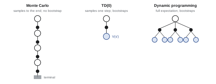
TD learning combines the sampling of MC with the bootstrapping of DP. After each step, TD(0) updates the value of the state just left toward the reward received plus the discounted current estimate of the next state:

The bracketed quantity, \(\delta_t = R_{t+1} + \gamma V(S_{t+1}) - V(S_t)\), is the TD error: the difference between the estimate made one step later and the earlier estimate. TD learns from each transition as it happens, without waiting for the episode to end and without a model. Its target uses an estimate, so it is biased early in learning, but it has much lower variance than the MC return because it depends on only one random reward and transition.

A neat illustration is predicting travel time home. Leaving the office you estimate 30 minutes; at the car, seeing rain, you revise to 40; on the highway, traffic is light and you revise to 35. A Monte Carlo learner adjusts its estimate at the office only after arriving home; a TD learner adjusts it immediately when it sees the rain, using the revised prediction as the target. TD error signals of this kind also match the firing of dopamine neurons in the brain, which respond to unexpected changes in predicted reward.

import numpy as np

# Random walk: states A..E (1..5), terminals 0 (reward 0) and 6 (reward 1); start at C.
true_v = np.arange(1, 6) / 6
rng = np.random.default_rng(1)

def episode():
    s, traj = 3, [3]
    while 0 < s < 6:
        s += 1 if rng.random() < 0.5 else -1
        traj.append(s)
    return traj, 1.0 if s == 6 else 0.0

def rms_after(method, alpha, n_episodes=100, runs=100):
    errs = []
    for _ in range(runs):
        V = np.full(7, 0.5); V[0] = V[6] = 0.0
        for _ in range(n_episodes):
            traj, G = episode()
            if method == "MC":                              # every-visit constant-alpha MC
                for s in traj[:-1]:
                    V[s] += alpha * (G - V[s])
            else:                                           # TD(0)
                for s, s2 in zip(traj[:-1], traj[1:]):
                    r = 1.0 if s2 == 6 else 0.0
                    V[s] += alpha * (r + V[s2] - V[s])
        errs.append(np.sqrt(np.mean((V[1:6] - true_v) ** 2)))
    return np.mean(errs)

for alpha in [0.01, 0.03, 0.05, 0.1]:
    mc, td = rms_after("MC", alpha), rms_after("TD", alpha)
    print(f"alpha = {alpha:4.2f}:  RMS error after 100 episodes   MC {mc:.3f}   TD(0) {td:.3f}")

alpha = 0.01:  RMS error after 100 episodes   MC 0.094   TD(0) 0.128
alpha = 0.03:  RMS error after 100 episodes   MC 0.097   TD(0) 0.039
alpha = 0.05:  RMS error after 100 episodes   MC 0.128   TD(0) 0.035
alpha = 0.10:  RMS error after 100 episodes   MC 0.172   TD(0) 0.055

For every step size except the smallest, TD(0) is much more accurate than Monte Carlo after 100 episodes; the best TD error is about a third of the best MC error. The smallest step size is too slow for TD to propagate values across the chain in 100 episodes, while larger step sizes make MC noisier because its targets have high variance. On many problems TD learns faster than MC, though neither dominates universally.

Batch learning and certainty equivalence

Given a fixed batch of experience, repeatedly applying the updates until convergence makes MC and TD converge to different answers. Batch MC finds the values that minimize squared error on the observed returns. Batch TD finds the values that would be exactly correct for the maximum likelihood model of the MDP estimated from the data, called the certainty-equivalence estimate. When the Markov property holds, the TD answer generalizes better to new data, which explains its advantage.

n-step methods and eligibility traces

MC and TD(0) are two ends of a spectrum. An \(n\)-step return uses \(n\) actual rewards and then bootstraps:

TD(0) is the 1-step case, and MC the case where \(n\) reaches the end of the episode. Intermediate values of \(n\) often learn fastest, trading variance against bias. TD(λ) averages all \(n\)-step returns with weights proportional to \(\lambda^{n-1}\), and can be implemented efficiently with eligibility traces, which keep a decaying record of recently visited states so that each TD error updates all of them in proportion to their recency. \(\lambda = 0\) gives TD(0) and \(\lambda = 1\) behaves like MC. Generalized advantage estimation in modern policy gradient methods (Lesson 9) is the same idea.

SARSA: on-policy TD control

For control, TD methods learn action values. SARSA updates \(Q(S_t, A_t)\) toward the reward plus the value of the next state-action pair actually chosen by the current policy:

The name comes from the quintuple \((S_t, A_t, R_{t+1}, S_{t+1}, A_{t+1})\) used in each update. The policy is ε-greedy with respect to \(Q\), so evaluation and improvement happen together at every step (GPI at its finest grain). SARSA is on-policy: it learns the value of the policy it actually follows, including its exploration. It converges to an optimal policy if all state-action pairs are visited infinitely often and the policy becomes greedy in the limit, for example by decaying ε.

Q-learning: off-policy TD control

Q-learning, introduced by Chris Watkins in 1989, replaces the value of the next action actually taken with the value of the best next action:

This update estimates \(q_*\) directly, regardless of the policy used to generate the experience, so Q-learning is off-policy: it can learn the optimal greedy policy while behaving exploratorily, and even from experience generated by other agents or from logged data. It converges to \(q_*\) with probability 1 under standard conditions on step sizes and exploration. Q-learning is simple and powerful, and with neural networks it became the deep Q-network of Lesson 7.

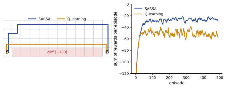
The difference between on-policy and off-policy learning shows clearly on the cliff-walking task: an agent must cross a grid from start to goal along the edge of a cliff, with −1 per step and −100 for falling off, which also sends it back to the start.

import numpy as np

# Cliff walking: 4 x 12 grid, start bottom-left, goal bottom-right, the cells between are a cliff.
H, W = 4, 12
start, goal = (3, 0), (3, 11)
acts = [(-1, 0), (1, 0), (0, -1), (0, 1)]

def step(s, a):
    r, c = s[0] + acts[a][0], s[1] + acts[a][1]
    r, c = min(max(r, 0), H - 1), min(max(c, 0), W - 1)
    if r == 3 and 0 < c < 11:
        return start, -100.0, False                 # fell off the cliff
    return (r, c), -1.0, (r, c) == goal

def train(method, episodes=500, alpha=0.5, eps=0.1, seed=0):
    rng = np.random.default_rng(seed)
    Q = np.zeros((H, W, 4)); returns = []
    pick = lambda s: int(rng.integers(4)) if rng.random() < eps else int(np.argmax(Q[s]))
    for _ in range(episodes):
        s = start; a = pick(s); total = 0.0
        for _ in range(1000):
            s2, r, done = step(s, a); total += r
            a2 = pick(s2)
            target = r if done else r + (Q[s2][a2] if method == "SARSA" else Q[s2].max())
            Q[s][a] += alpha * (target - Q[s][a])
            s, a = s2, a2
            if done:
                break
        returns.append(total)
    return Q, np.array(returns)

def greedy_path(Q):
    s, path = start, [start]
    for _ in range(50):
        s, _, done = step(s, int(np.argmax(Q[s])))
        path.append(s)
        if done:
            break
    return path

for method in ["SARSA", "Q-learning"]:
    runs = [train(method, seed=k) for k in range(20)]
    avg = np.mean([ret[-100:].mean() for _, ret in runs])
    print(f"{method}: average return per episode while learning (last 100 episodes, 20 runs) = {avg:.1f}")
    path = set(greedy_path(runs[2][0]))
    for r in range(H):
        row = ""
        for c in range(W):
            row += "S" if (r, c) == start else "G" if (r, c) == goal else "o" if (r, c) in path else "C" if r == 3 else "."
        print("   " + row)

SARSA: average return per episode while learning (last 100 episodes, 20 runs) = -26.3
   .ooooooooooo
   oo.........o
   o..........o
   SCCCCCCCCCCG
Q-learning: average return per episode while learning (last 100 episodes, 20 runs) = -53.2
   ............
   ............
   oooooooooooo
   SCCCCCCCCCCG

Q-learning learns the optimal path, straight along the cliff edge (13 steps), because it evaluates the greedy policy. But while it is still exploring with ε = 0.1, its random actions occasionally send it over the cliff, so its average return during learning is about −53. SARSA learns the value of the ε-greedy policy it actually follows, including the risk of random steps near the edge, so it prefers a safer path along the top of the grid: longer, but with an average return of about −26 during learning. Which is better depends on whether performance during learning matters: an online system that must explore with real consequences may prefer SARSA's caution.

Maximization bias and double learning

Q-learning's target takes a maximum over noisy estimates, and the maximum of noisy estimates is biased upward: if all actions truly have value 0 but estimates are noisy, the largest estimate is positive. This maximization bias can make Q-learning overestimate values and prefer actions with uncertain estimates. Double Q-learning fixes it by keeping two independent estimates, using one to choose the maximizing action and the other to evaluate it: \(Q_1(S_t, A_t) \leftarrow Q_1 + \alpha[R + \gamma Q_2(S_{t+1}, \arg\max_a Q_1(S_{t+1}, a)) - Q_1]\), alternating roles. Double DQN uses the same idea with neural networks.

Lesson 6 combines these learning methods with planning in Dyna and Monte Carlo tree search, and Lesson 7 extends them to function approximation.