Exploration and distributional reinforcement learning

Lesson 7 introduced deep Q-networks and listed the improvements that followed. Two of those directions deserve a closer look because they address limitations that remain central to modern reinforcement learning. The first is exploration: ε-greedy and similar dithering strategies work when rewards are easy to stumble upon, but fail completely in problems where reaching a reward requires a long, specific sequence of actions. The second is distributional RL: instead of learning only the expected return, learn the whole distribution of returns, which turns out to improve learning even when only the mean is used and gives risk information when it matters. This lesson treats both, then shows how the improvements combine in the Rainbow agent, and closes with practical advice on evaluating deep RL agents fairly.

Why dithering exploration fails

An ε-greedy agent explores by taking random actions occasionally. To reach a reward that requires \(N\) specific consecutive actions, a random walk needs on the order of \(2^N\) attempts or more, so the time to find a reward grows exponentially with how deep it lies. In the Atari game Montezuma's Revenge, the first reward requires navigating ladders, ropes and enemies for hundreds of steps; DQN scored almost nothing on it for this reason.

Deep exploration means committing to exploratory behaviour for many consecutive steps, driven by the agent's uncertainty about long-term consequences rather than by noise added to each action. The bandit principle of optimism in the face of uncertainty (Lesson 2) extends to sequential problems: if the agent values unfamiliar states optimistically, it will plan its way toward them deliberately.

import numpy as np

# A chain of N states. "Right" moves one step right and gives a tiny cost; "left" returns to state 0
# with reward 0.01 (a distracting small reward). Only reaching the far end pays +10 (episode ends), so going right is optimal.
def episode_to_find_goal(N, method, max_eps=2000, seed=0):
    rng = np.random.default_rng(seed)
    Q = np.zeros((N, 2)) if method == "eps-greedy" else np.full((N, 2), 2.0)   # optimism for the bonus agent
    counts = np.zeros((N, 2))
    for ep in range(1, max_eps + 1):
        s = 0
        for t in range(N + 10):
            if method == "eps-greedy":
                a = int(rng.integers(2)) if rng.random() < 0.1 else int(np.argmax(Q[s] + 1e-9 * rng.random(2)))
            else:                                       # UCB-style: value plus a bonus that shrinks with visits
                a = int(np.argmax(Q[s] + 0.1 / np.sqrt(counts[s] + 1) + 1e-9 * rng.random(2)))
            counts[s, a] += 1
            if a == 1:
                s2, r = s + 1, -0.001
            else:
                s2, r = 0, 0.01
            if s2 == N - 1:
                return ep
            bonus = 0.1 / np.sqrt(counts[s, a]) if method == "count bonus" else 0.0   # intrinsic reward
            target = r + bonus + 0.99 * Q[s2].max()
            Q[s, a] += 0.2 * (target - Q[s, a])
            s = s2
    return None

for N in (10, 20, 40):
    for m in ("eps-greedy", "count bonus"):
        res = [episode_to_find_goal(N, m, seed=k) for k in range(10)]
        found = [r for r in res if r is not None]
        txt = f"median {int(np.median(found))} episodes" if found else "never"
        print(f"chain length {N:2d}, {m:11s}: goal found in {len(found)}/10 runs, {txt}")

chain length 10, eps-greedy : goal found in 1/10 runs, median 1317 episodes
chain length 10, count bonus: goal found in 10/10 runs, median 51 episodes
chain length 20, eps-greedy : goal found in 0/10 runs, never
chain length 20, count bonus: goal found in 10/10 runs, median 71 episodes
chain length 40, eps-greedy : goal found in 0/10 runs, never
chain length 40, count bonus: goal found in 10/10 runs, median 82 episodes

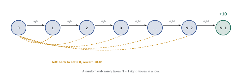
ε-greedy found the goal in only one of ten runs of the shortest chain and never in the longer ones: the small reward for returning to the start keeps it near the beginning, and the chance of a long run of right moves is tiny. The agent with optimistic initial values and a count-based bonus explores systematically, because every unvisited state looks valuable until tried, and finds the goal in every run, with the number of episodes growing only slowly with chain length.

Exploration bonuses in large state spaces

In a table, visit counts are easy. In large or continuous state spaces, every state is new, so methods approximate novelty in other ways and add it as an intrinsic reward \(r^+\) to the environment reward:

• Pseudo-counts derive a count-like quantity from a density model of visited states: states the model assigns low probability get large bonuses, typically \(\beta/\sqrt{\hat N(s)}\).
• Random network distillation (RND) trains a predictor network to match the output of a fixed, randomly initialized target network on visited states. Prediction error is high for unfamiliar states and falls as they are visited, giving a simple novelty signal. RND was the first method to exceed average human performance on Montezuma's Revenge without demonstrations.
• Curiosity based on prediction error rewards transitions whose consequences the agent's forward model predicts poorly, encouraging it to learn about its environment. A known failure is the "noisy TV" problem: an agent rewarded for unpredictability can become fixated on inherently random sources such as a screen of static. Predicting in a learned feature space that ignores irrelevant details, or rewarding learning progress rather than raw error, reduces this.
• Go-Explore remembers promising states, returns to them (by resetting a simulator or with a goal-conditioned policy) and explores from there, solving hard-exploration Atari games by separating the problems of returning and exploring.

Intrinsic rewards change the objective, so they are usually scaled down over training or kept in a separate value head, and the final policy is evaluated on the environment reward alone.

Exploration by uncertainty: posterior sampling

Thompson sampling (Lesson 2) extends to full RL as posterior sampling: sample one plausible model or value function from the posterior, act greedily with respect to it for a whole episode, then update. Because the sample is held fixed for the episode, the agent commits to exploring one hypothesis deeply rather than dithering. With neural networks, exact posteriors are unavailable, but approximations work well. Bootstrapped DQN trains several Q-value heads on different bootstrap samples of the data and selects one at random each episode; randomized prior functions add a fixed random network to each head so that ensemble members disagree in unexplored regions. These methods scale exploration to deep RL without hand-designed bonuses.

Distributional reinforcement learning

The return from a state is a random variable: it depends on random transitions, rewards and future actions. Standard value-based methods learn only its expectation, \(Q(s, a) = \mathbb{E}[G \mid s, a]\). Distributional RL learns the full distribution \(Z(s, a)\), satisfying a distributional Bellman equation:

where \(\overset{D}{=}\) means equality in distribution. The distribution of returns from \((s, a)\) is the distribution of the immediate reward plus the discounted return from the next state.

The C51 algorithm represents each distribution as probabilities on a fixed set of 51 atoms (support points) between a minimum and maximum return. To form the learning target, each atom of the next state's distribution is shifted by the reward and shrunk by \(\gamma\), which moves it between atoms, so its probability mass is split between the two nearest atoms (a projection). The network is trained to minimize the cross-entropy between its predicted distribution and the projected target.

import numpy as np

# Categorical (C51-style) distributional Bellman update with 11 atoms on [-10, 10]
atoms = np.linspace(-10, 10, 11)
dz = atoms[1] - atoms[0]
next_dist = np.zeros(11); next_dist[[3, 8]] = [0.5, 0.5]      # bimodal next-state return: -4 or +6
r, gamma = 1.0, 0.9

def project(r, gamma, p):
    target = np.clip(r + gamma * atoms, atoms[0], atoms[-1])   # shift and shrink each atom
    out = np.zeros(11)
    for tz, prob in zip(target, p):
        b = (tz - atoms[0]) / dz
        lo, hi = int(np.floor(b)), int(np.ceil(b))
        if lo == hi: out[lo] += prob
        else:
            out[lo] += prob * (hi - b); out[hi] += prob * (b - lo)   # split mass between neighbours
    return out

new = project(r, gamma, next_dist)
print("atoms:     ", atoms)
print("projected: ", np.round(new, 3))
print(f"mean of target distribution {new @ atoms:.2f} (should equal r + gamma * mean = {r + gamma * (next_dist @ atoms):.2f})")
print(f"probability the return is negative: {new[atoms < 0].sum():.2f}; a mean-only method sees just {new @ atoms:.2f}")

atoms:      [-10.  -8.  -6.  -4.  -2.   0.   2.   4.   6.   8.  10.]
projected:  [0.   0.   0.   0.15 0.35 0.   0.   0.   0.4  0.1  0.  ]
mean of target distribution 1.90 (should equal r + gamma * mean = 1.90)
probability the return is negative: 0.50; a mean-only method sees just 1.90

The projected distribution preserves the mean exactly (1.90 in both calculations) while keeping the two modes: half the probability lies on negative returns. An agent that knows only the mean of 1.9 cannot tell this action from one that reliably returns 1.9, a difference that matters greatly for risk-sensitive decisions.

Quantile regression DQN (QR-DQN) and implicit quantile networks (IQN) instead learn the returns at fixed or sampled quantile levels, avoiding a fixed support and the projection. Empirically, distributional methods improve performance even when the agent acts on the mean, probably because predicting a whole distribution provides a richer learning signal and more stable representations. The learned distributions also enable risk-sensitive policies, for example maximizing a low quantile or the conditional value at risk (the mean of the worst outcomes), useful in finance, safety-critical control and anywhere bad outcomes are much worse than average ones are good.

Rainbow: combining improvements

The Rainbow agent (2017) combined six extensions to DQN: double Q-learning, prioritized replay, dueling networks, multi-step returns, distributional (C51) learning and noisy networks for exploration (which learn parameterized noise in the weights instead of using ε-greedy). On the 57-game Atari benchmark, Rainbow reached in about 7 million frames the median performance DQN achieved in 200 million, and finished far higher. Ablation studies, removing one component at a time, found prioritized replay and multi-step returns most important, followed by distributional learning; the others contributed less but were still useful.

Later agents pushed further, using recurrent networks with large-scale distributed replay (R2D2), meta-learned exploration strategies across a family of policies with different exploration levels (Agent57, the first to exceed the human benchmark on all 57 games), and model-based planning (MuZero, Lesson 6). The general lesson from this line of work is that many independent improvements, each modest, compound into large gains, but also that results depend on careful engineering choices that are easy to overlook.

Evaluating deep RL agents fairly

Deep RL results are notoriously variable. Performance can differ dramatically between random seeds of the same algorithm, and small implementation details (reward scaling, observation normalization, network initialization, how episode time limits are handled) can matter as much as the algorithm itself. Good evaluation practice includes:

• Report results over many seeds (often 5 to 10 or more) with confidence intervals, not the best run.
• Use robust aggregate measures across tasks, such as the interquartile mean of normalized scores, and performance profiles showing the fraction of runs above each score.
• Tune baselines with the same effort as the proposed method.
• Separate the evaluation policy (usually greedy or low-noise) from the training policy, and evaluate on held-out levels or seeds for procedurally generated environments, to test generalization rather than memorization.
• Report sample efficiency (performance against environment steps) and computational cost, not only final performance.