Planning and learning: Dyna and Monte Carlo tree search

Dynamic programming (Lesson 3) plans with a complete model of the environment; Monte Carlo and temporal-difference methods (Lesson 5) learn from experience with no model at all. Between these extremes lie methods that learn a model from experience and use it to plan, and methods that plan at the moment of decision by simulating possible futures. Combining learning and planning lets an agent squeeze far more value from each real interaction, which matters whenever real experience is slow, costly or risky. This lesson covers models and planning, the Dyna architecture, prioritized sweeping, decision-time planning with rollouts and Monte Carlo tree search, and the AlphaZero and MuZero systems that combined tree search with deep learning to master board games and Atari.

Models and planning

A model is anything the agent can use to predict how the environment will respond to its actions. Distribution models give the full probabilities \(p(s', r \mid s, a)\), as dynamic programming requires; sample models produce one possible outcome at a time, like a simulator. Sample models are easier to build and are enough for most planning methods.

Planning, in this sense, means using a model to improve a policy or value function without interacting with the real environment. A unifying view is that planning and learning do the same thing, updating values toward targets, but with different sources of experience: real transitions for learning, simulated transitions for planning. The same update rules serve both.

Models can be given (the rules of chess, a physics simulator, a factory's digital twin) or learned from data. Learned models are imperfect, and a policy that exploits a model's errors can look excellent in simulation and fail in reality, a central difficulty of model-based reinforcement learning (Lesson 10).

Dyna: integrating learning and planning

Dyna, proposed by Sutton in 1990, interleaves three processes in one agent:

• Direct reinforcement learning: update values from each real transition, for example with Q-learning.
• Model learning: record each real transition in a model; in a deterministic tabular world, simply remember that taking \(a\) in \(s\) led to \(s'\) with reward \(r\).
• Planning: after each real step, perform \(n\) simulated updates by sampling previously visited state-action pairs, asking the model what happens, and applying the same Q-learning update.

Each real step thus produces \(n + 1\) value updates. When rewards are discovered, planning propagates them backward through the remembered transitions much faster than real experience alone could.

import numpy as np

# 6 x 9 maze (Sutton and Barto style). Walls block some cells; start S, goal G gives +1.
H, W = 6, 9
walls = {(1, 2), (2, 2), (3, 2), (4, 5), (0, 7), (1, 7), (2, 7)}
start, goal = (2, 0), (0, 8)
moves = [(-1, 0), (1, 0), (0, -1), (0, 1)]
def step(s, a):
    r, c = s[0] + moves[a][0], s[1] + moves[a][1]
    if not (0 <= r < H and 0 <= c < W) or (r, c) in walls: r, c = s
    return (r, c), (1.0 if (r, c) == goal else 0.0)

def dyna(n_plan, episodes=30, seed=0):
    rng = np.random.default_rng(seed)
    Q = np.zeros((H, W, 4)); model = {}; steps = []
    for ep in range(episodes):
        s, n = start, 0
        while s != goal:
            a = int(rng.integers(4)) if rng.random() < 0.1 else int(np.argmax(Q[s] + 1e-6 * rng.random(4)))
            s2, r = step(s, a)
            Q[s][a] += 0.1 * (r + 0.95 * Q[s2].max() * (s2 != goal) - Q[s][a])
            model[(s, a)] = (s2, r)
            keys = list(model)
            for _ in range(n_plan):                     # planning: replay simulated experience from the model
                ps, pa = keys[rng.integers(len(keys))]
                ps2, pr = model[(ps, pa)]
                Q[ps][pa] += 0.1 * (pr + 0.95 * Q[ps2].max() * (ps2 != goal) - Q[ps][pa])
            s, n = s2, n + 1
        steps.append(n)
    return steps

for n_plan in (0, 5, 50):
    runs = np.array([dyna(n_plan, seed=k) for k in range(10)])
    m = runs.mean(0)
    print(f"{n_plan:2d} planning steps per real step: steps per episode, episodes 2-5: {np.round(m[1:5]).astype(int)}, episode 30: {m[-1]:.0f}")

 0 planning steps per real step: steps per episode, episodes 2-5: [530 736 412 301], episode 30: 48
 5 planning steps per real step: steps per episode, episodes 2-5: [173  96  53  56], episode 30: 16
50 planning steps per real step: steps per episode, episodes 2-5: [57 28 17 18], episode 30: 17

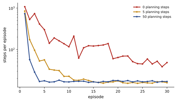
Without planning, the agent needs dozens of episodes to learn a short path; with 50 planning steps per real step, it finds a near-optimal path in about three episodes. Each real experience is reused many times. The price is computation: 50 planning updates per step cost 50 times the arithmetic, which is cheap compared with real interaction in robotics, industrial control or anything involving people.

When the environment changes, a model can become wrong. If a shortcut opens, a model built from past experience will never suggest exploring it. Dyna-Q+ adds an exploration bonus for state-action pairs not tried recently, \(r + \kappa\sqrt{\tau}\), where \(\tau\) is the time since the pair was last tried, encouraging the agent to test whether its model is still correct.

Prioritized sweeping

Uniformly sampling remembered transitions for planning wastes effort, because most updates change nothing: early in learning, most values are zero, and updating a zero from another zero achieves nothing. Prioritized sweeping focuses planning where it matters. When a value changes by a large amount, the predecessors of that state, the state-action pairs that lead to it, are placed in a priority queue ordered by how much their values would change. Planning updates the highest-priority pairs first, which propagates new information backward efficiently, like a wave spreading from the place where a reward was found. In large problems prioritized sweeping can reduce planning computation by orders of magnitude. The same idea, prioritizing by the size of the TD error, underlies prioritized experience replay in deep RL (Lesson 8).

Decision-time planning

Dyna performs background planning, improving a value function or policy used for all future decisions. Decision-time planning instead focuses computation on the current state: when a decision must be made, simulate possible futures from here, choose the best action, and discard most of the computation. It suits problems where the model is accurate and the state space too vast to cover in advance, such as games.

The simplest form is the rollout algorithm: for each available action, simulate many trajectories that begin with that action and then follow a simple rollout policy (often random), average their returns, and pick the action with the highest average. Rollouts improve on the rollout policy, by the policy improvement theorem of Lesson 3, but spend equal effort on promising and hopeless actions.

Monte Carlo tree search

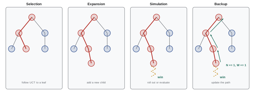
Monte Carlo tree search (MCTS) builds a search tree from the current state incrementally, directing simulations toward the most promising lines while still exploring others. Each iteration has four phases:

• Selection: starting at the root, descend the tree by choosing actions with a bandit rule, until reaching a node that has not been fully expanded.
• Expansion: add one or more child nodes for untried actions.
• Simulation (evaluation): estimate the value of the new node, classically by a random rollout to the end of the game, or, in modern systems, by a learned value network.
• Backup: propagate the result up the path to the root, updating visit counts and value estimates at every node on the way.

The most common selection rule is UCT (upper confidence bounds applied to trees), which treats each node's choice as a bandit (Lesson 2):

where \(N(s)\) is the number of visits to the node and \(N(s, a)\) the visits to the child. After the search, the action taken is usually the most visited child, which is more robust than the one with the highest average.

import numpy as np

# Nim: take 1, 2 or 3 stones; whoever takes the last stone wins. Monte Carlo tree search with UCT.
rng = np.random.default_rng(6)
class Node:
    def __init__(self, stones):
        self.stones, self.N, self.W, self.children = stones, 0, 0.0, {}   # W: wins for the player to move here

def rollout(stones):
    """Random play to the end; returns 1 if the player to move now wins."""
    player = 0
    while True:
        stones -= int(rng.integers(1, min(3, stones) + 1))
        if stones == 0: return 1.0 if player == 0 else 0.0
        player = 1 - player

def search(node):
    if node.stones == 0:
        v = 0.0                                       # no stones left: the player to move has lost
    elif node.N == 0:
        v = rollout(node.stones)                      # new leaf: estimate its value by a random rollout
    else:
        for m in (1, 2, 3):
            if m <= node.stones and m not in node.children: node.children[m] = Node(node.stones - m)
        def uct(k):
            c = node.children[k]
            if c.N == 0: return float("inf")
            return (1 - c.W / c.N) + 1.4 * np.sqrt(np.log(node.N) / c.N)   # value for the player choosing
        m = max(node.children, key=uct)
        v = 1.0 - search(node.children[m])
    node.N += 1; node.W += v
    return v

for stones in (10, 13, 15, 16):
    root = Node(stones)
    for _ in range(5000): search(root)
    visits = {m: c.N for m, c in root.children.items()}
    best = max(visits, key=visits.get)
    print(f"{stones} stones: visits {visits}; MCTS takes {best}, leaving {stones - best}; estimated win probability {1 - root.children[best].W / root.children[best].N:.2f}")

10 stones: visits {1: 163, 2: 4801, 3: 35}; MCTS takes 2, leaving 8; estimated win probability 0.96
13 stones: visits {1: 4515, 2: 224, 3: 260}; MCTS takes 1, leaving 12; estimated win probability 0.86
15 stones: visits {1: 812, 2: 575, 3: 3612}; MCTS takes 3, leaving 12; estimated win probability 0.83
16 stones: visits {1: 1766, 2: 1847, 3: 1386}; MCTS takes 2, leaving 14; estimated win probability 0.48

The winning strategy in this game is to leave the opponent a multiple of four stones. With 10, 13 and 15 stones, MCTS concentrates its visits on exactly the move that does this, discovering the strategy from random rollouts alone. With 16 stones every move loses against perfect play, and the search spreads its visits among the three moves, estimating about even chances only because its rollouts assume a random opponent.

MCTS needs no evaluation function and works with only a sample model, which made it the breakthrough method for computer Go in the late 2000s, where hand-crafted evaluation had failed. It is also used for planning in POMDPs from the current belief (Lesson 4), for scheduling and combinatorial optimization, and for search over reasoning steps in language models.

AlphaZero and MuZero

AlphaGo (2016) defeated a world champion at Go by combining MCTS with deep neural networks: a policy network to suggest promising moves and a value network to evaluate positions, trained first on human games and then by self-play reinforcement learning. AlphaZero (2017) removed the human data entirely and mastered Go, chess and shogi from the rules alone. Its training loop is a clear example of planning and learning working together:

• A single network outputs a policy \(\mathbf{p}\) (move probabilities) and a value \(v\) (expected outcome) for any position.
• Self-play games are generated with MCTS, which uses \(\mathbf{p}\) as a prior to focus selection (the PUCT rule, \(\bar Q + c\,p(a)\sqrt{N(s)}/(1 + N(s, a))\)) and \(v\) in place of random rollouts.
• The network is trained to predict the MCTS visit distribution (which is a better policy than \(\mathbf{p}\), because search improves on it) and the final game outcome.
• The improved network makes the next round of search stronger, and so on: search acts as a policy improvement operator, and learning distils the improved policy back into the network.

MuZero (2019) went further by learning the model itself. Instead of using the game rules, it learns a representation function that encodes an observation into a hidden state, a dynamics function that predicts the next hidden state and reward from a hidden state and action, and a prediction function giving the policy and value. MCTS then plans entirely inside this learned latent space. The model is trained only to predict the quantities planning needs (rewards, values and policies), not to reconstruct observations, which made MuZero effective on visually complex Atari games as well as board games. Its descendants have been applied to video compression and code optimization.