Function approximation and deep RL

The tabular methods of Lessons 3 and 5 store a separate value for every state or state-action pair. That is impossible when states are numerous or continuous: the positions and velocities of a robot's joints, the pixels of a video game screen, the temperatures and flows of a cooling plant. Even if a table could be stored, most states would never be visited, so the agent must generalize from the states it has seen to similar ones it has not. Function approximation replaces the table with a parameterized function, from linear models on hand-designed features to deep neural networks. This lesson covers value function approximation, the gradient-based learning rules, feature construction, the stability problems known as the deadly triad, deep Q-networks and their refinements, and model-based and offline RL.

Value function approximation

The value function is represented as \(\hat v(s, \mathbf w)\) with a weight vector \(\mathbf w\) much smaller than the number of states. Changing one weight changes the estimated values of many states, which is how the approximation generalizes, and also why it cannot be exact everywhere. The natural objective is the mean squared value error, weighted by how often each state is visited under the policy, \(\mu(s)\):

Stochastic gradient descent on this objective, with the unknown \(v_\pi(S_t)\) replaced by a target \(U_t\), gives the update

With the Monte Carlo return as the target, \(U_t = G_t\), this is true stochastic gradient descent and converges to a local minimum of the value error. With the TD target \(U_t = R_{t+1} + \gamma\hat v(S_{t+1}, \mathbf w)\), the target itself depends on \(\mathbf w\), but the update ignores that dependence; it is therefore called semi-gradient TD. Semi-gradient methods are not true gradient methods, but they usually learn faster and work online, and for linear approximation with on-policy data they converge reliably.

Linear methods

In linear function approximation, each state is described by a feature vector \(\mathbf x(s)\) and \(\hat v(s, \mathbf w) = \mathbf w^\top\mathbf x(s)\), so the gradient is simply \(\mathbf x(s)\). Linear semi-gradient TD(0) converges, on-policy, to the TD fixed point, whose value error is at most \(1/(1 - \gamma)\) times the smallest error achievable by any weight vector. The quality of the result therefore depends on the features:

• State aggregation groups states and gives each group one weight: a one-hot feature for the group.
• Tile coding overlays several offset grids (tilings) on a continuous state space; each state activates one tile per tiling, giving a sparse binary feature vector that generalizes to nearby states and is very cheap to compute. It was the workhorse of RL for robotics and control before deep learning.
• Radial basis functions, polynomial and Fourier bases give smooth features.
• Learned features from neural networks, the subject of deep RL.

import numpy as np

# 1000-state random walk: start in the middle, jump uniformly 1 to 100 states left or right;
# leaving on the left gives reward -1, on the right +1. Undiscounted.
N = 1000
P = np.zeros((N, N)); b = np.zeros(N)
for s in range(N):
    for d in list(range(-100, 0)) + list(range(1, 101)):
        s2 = s + d
        if s2 < 0: b[s] += -1 / 200
        elif s2 >= N: b[s] += 1 / 200
        else: P[s, s2] += 1 / 200
true_v = np.linalg.solve(np.eye(N) - P, b)          # exact values for comparison

rng = np.random.default_rng(0)
def run_td(groups, episodes=3000, alpha=0.01):
    w = np.zeros(groups); size = N // groups
    for _ in range(episodes):
        s = 500
        while True:
            d = int(rng.integers(1, 101)) * (1 if rng.random() < 0.5 else -1)
            s2 = s + d
            g = s // size
            if s2 < 0 or s2 >= N:
                r = -1.0 if s2 < 0 else 1.0
                w[g] += alpha * (r - w[g])
                break
            w[g] += alpha * (w[s2 // size] - w[g])      # semi-gradient TD(0) with one-hot group features
            s = s2
    return np.repeat(w, size)

for groups in [5, 10, 50]:
    v = run_td(groups)
    print(f"{groups:3d} groups ({groups} weights): RMS error vs true values = {np.sqrt(np.mean((v - true_v) ** 2)):.3f}")
print(f"true values at states 100, 500, 900: {true_v[100]:.3f}, {true_v[500]:.3f}, {true_v[900]:.3f}")

  5 groups (5 weights): RMS error vs true values = 0.294
 10 groups (10 weights): RMS error vs true values = 0.137
 50 groups (50 weights): RMS error vs true values = 0.089
true values at states 100, 500, 900: -0.752, 0.001, 0.754

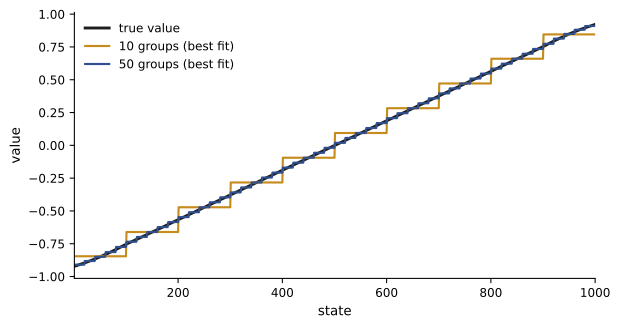
With only five groups, each weight covers 200 states whose true values range widely, so the approximation is coarse. Ten and fifty groups reduce the error considerably, at the cost of more weights to learn. Within each group the estimate is a constant, a staircase approximation of the smooth true value function; better features, such as tile coding or polynomials, would fit the curve with few weights.

Control with function approximation

For control, the action-value function is approximated as \(\hat q(s, a, \mathbf w)\), and semi-gradient SARSA or Q-learning updates \(\mathbf w\) with the corresponding TD errors. For discrete actions, a network often outputs one value per action from the state. For continuous actions, maximizing over actions is itself an optimization problem, which is one reason continuous control uses actor-critic methods (Lesson 9).

The deadly triad

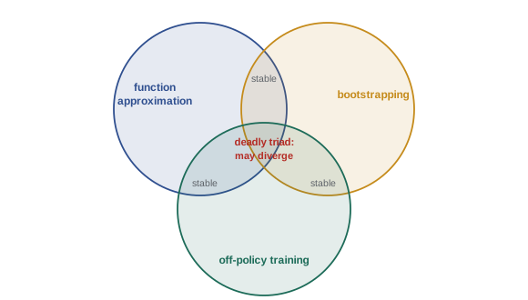
Combining three ingredients can make learning unstable, with values diverging to infinity even in simple problems:

• Function approximation, which generalizes across states.
• Bootstrapping, which updates toward targets built from current estimates.
• Off-policy training, in which the distribution of updates differs from the distribution the target policy would generate.

Any two are safe: tabular methods can bootstrap off-policy, Monte Carlo with function approximation does not bootstrap, and on-policy linear TD converges. All three together can diverge. The classic demonstration is Baird's counterexample, a seven-state MDP with all rewards zero, where the correct answer is trivially zero values, yet off-policy semi-gradient TD drives the weights to infinity.

import numpy as np

# Baird counterexample: 7 states, 8 weights, all rewards zero, so the true values are all 0.
X = np.zeros((7, 8))
for i in range(6):
    X[i, i] = 2; X[i, 7] = 1                  # upper states: v = 2 w_i + w_8
X[6, 6] = 1; X[6, 7] = 2                      # lower state:  v = w_7 + 2 w_8
gamma, alpha = 0.99, 0.01
w0 = np.array([1, 1, 1, 1, 1, 1, 10, 1], float)

def expected_td(off_policy, sweeps=1000):
    w = w0.copy()
    for k in range(1, sweeps + 1):
        v = X @ w
        if off_policy:
            # behaviour: uniform over states; target policy always goes to the lower state (7);
            # importance ratio is 7 for the solid action, 0 for dashed, solid chosen with prob 1/7
            delta = gamma * v[6] - v                 # TD error under the target policy
            w += alpha * (X.T @ delta) / 7           # semi-gradient, states weighted uniformly
        else:
            # on-policy: states visited in proportion to the target policy (all mass on state 7)
            delta = gamma * v[6] - v[6]
            w += alpha * delta * X[6]
        if k in (1, 10, 100, 1000):
            tag = "off" if off_policy else "on "
            print(f"{tag}-policy, sweep {k:4d}: |w| = {np.linalg.norm(w):12.2f}")
expected_td(True)
expected_td(False)

off-policy, sweep    1: |w| =        10.37
off-policy, sweep   10: |w| =        10.61
off-policy, sweep  100: |w| =        16.83
off-policy, sweep 1000: |w| =       436.86
on -policy, sweep    1: |w| =        10.34
on -policy, sweep   10: |w| =        10.33
on -policy, sweep  100: |w| =        10.21
on -policy, sweep 1000: |w| =         9.42

Off-policy, the weight norm grows without bound even though every reward is zero, because updates are made from states the target policy never visits, and the generalization through shared weights then pushes up the value the target policy's own state bootstraps from. On-policy updates remain bounded. Remedies include gradient-TD methods that perform true gradient descent on a projected Bellman error, emphatic TD, and, in deep RL, the practical stabilizers of DQN described next.

Deep Q-networks

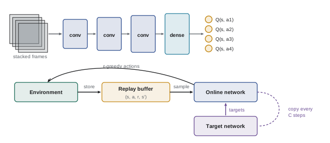
In 2015, the deep Q-network (DQN) learned to play 49 Atari 2600 games from raw pixels and the score, reaching human-level performance on many, with the same network architecture and hyperparameters for every game. DQN is Q-learning with a convolutional neural network approximating \(Q(s, a)\), and it confronts the deadly triad head-on. Two ideas made it work:

• Experience replay: transitions \((s, a, r, s')\) are stored in a large buffer (one million in the original), and each update uses a random mini-batch from it. This breaks the strong correlations between consecutive samples, which would otherwise violate the assumptions of stochastic gradient descent, and reuses each experience many times, improving data efficiency.
• Target network: the TD target is computed with a separate copy of the network whose weights \(\mathbf w^-\) are updated only periodically (every 10,000 steps in the original) or slowly averaged. This stops the target from chasing the network being trained, reducing oscillation and divergence.

The loss minimized for each mini-batch is

often with the Huber loss instead of the square to limit the effect of large errors, and with rewards clipped to a fixed range.

Improvements to DQN

• Double DQN uses the online network to choose the best next action and the target network to evaluate it, removing much of the maximization bias of Lesson 5.
• Dueling networks split the output into a state value and action advantages, \(Q(s, a) = V(s) + A(s, a) - \bar A(s)\), which helps when many actions have similar values.
• Prioritized replay samples transitions with large TD errors more often, with importance weights to correct the bias.
• Multi-step returns, distributional RL (learning the distribution of returns rather than its mean) and noisy networks for exploration.

The Rainbow agent combined these and roughly doubled DQN's median performance on Atari. Later agents reached superhuman scores on all 57 Atari games.

Model-based RL

Model-free methods can need millions of interactions. Model-based methods learn a model of the environment's dynamics and rewards from experience and use it to plan or to generate simulated experience. Dyna interleaves real steps with many simulated updates from the learned model. AlphaZero combines a learned value and policy network with Monte Carlo tree search using the known rules of chess and Go; MuZero extends this by learning the model itself in a latent space, reaching superhuman play in board games and strong Atari performance without knowing the rules. World-model approaches, such as the Dreamer agents, learn compact latent dynamics and train policies inside the model. Model-based methods are far more data-efficient, but model errors can be exploited by the planner, so they must be handled carefully.

Offline RL

In many applications, such as healthcare, industrial control or data centre operations, exploring with a poor policy on the real system is unacceptable, but large logs of past operation exist. Offline (batch) RL learns policies from such fixed datasets without further interaction. It is off-policy learning at its most extreme: naive Q-learning on logged data overestimates the values of actions the data never tried, because nothing corrects the errors. Offline methods therefore constrain the learned policy to stay close to the data (behaviour-regularized methods) or penalize values of unfamiliar actions (conservative Q-learning). Evaluating a new policy from logged data before deploying it, called off-policy evaluation, uses importance sampling (AI-320) and model-based estimates.

Practical deep RL

Deep RL is notoriously sensitive. Results can vary widely between random seeds, small implementation details matter, and rewards that are badly scaled or sparse slow learning drastically. Good practice is to normalize observations and rewards, start from well-tested implementations, report results over many seeds with confidence intervals, monitor value estimates for divergence, and begin with simple baselines. When a good simulator exists, massive parallel simulation makes many problems tractable; when it does not, model-based and offline methods and careful reward design matter most. Real deployments, such as RL-based control of data centre cooling, typically add safety constraints, human oversight and fallback to conventional controllers.

Lesson 8 develops two of the directions listed here, exploration and distributional RL, and Lesson 10 treats model-based and offline RL in depth.