Bandits in depth: regret, context and off-policy evaluation

Lesson 1 introduced the multi-armed bandit as the simplest setting where an agent must balance exploration and exploitation, and compared greedy, ε-greedy, UCB and Thompson sampling. Bandits are far more than a warm-up for full reinforcement learning: they run in production systems that choose which article, advertisement, product recommendation, notification or price to show, millions of times a day. This lesson develops the theory of regret, handles rewards that drift over time, adds context so that the best action can depend on who the user is, and treats the problem that matters most in practice: estimating how well a new policy would perform from data logged by an old one, without deploying it.

How small can regret be?

Regret measures the reward lost by not always choosing the best arm. A policy that explores at a fixed rate, like ε-greedy with constant ε, keeps choosing bad arms a fixed fraction of the time, so its regret grows linearly with the number of rounds \(T\). Good algorithms achieve regret that grows only logarithmically.

Lai and Robbins (1985) showed that this is the best possible. For any algorithm that performs reasonably on all problems, the number of times a suboptimal arm \(a\) is pulled must grow at least as

where the KL divergence (AI-320) measures how hard it is to distinguish arm \(a\)'s reward distribution from the best arm's. Arms that look almost as good as the best must be tried many times before they can be ruled out. Summing over arms, regret grows as \(\sum_a \Delta_a \ln T/\mathrm{KL}_a\), where \(\Delta_a\) is the gap between arm \(a\)'s mean and the best.

UCB1, which chooses \(\arg\max_a Q_t(a) + \sqrt{2\ln t/N_t(a)}\), achieves regret of order \(\sum_a (\ln T)/\Delta_a\), within a constant factor of the lower bound. Its confidence bonus comes from Hoeffding's inequality: with high probability, a true mean lies below the sample mean plus a term shrinking with the square root of the sample count. Thompson sampling matches the Lai-Robbins constant exactly for Bernoulli rewards, which, together with its simplicity, explains its popularity. When gaps can be arbitrarily small, the relevant measure is worst-case (minimax) regret, which for any algorithm is of order \(\sqrt{KT}\).

Rewards that change over time

Real environments drift: click rates change with news cycles, a product's appeal fades, prices respond to competitors. Stationary algorithms adapt poorly, because their sample averages give equal weight to old rewards and their confidence bonuses shrink until they stop exploring. Remedies include:

• A constant step size \(\alpha\), which turns the sample average into an exponentially weighted average with an effective memory of about \(1/\alpha\) observations (Lesson 1).
• Discounted or sliding-window UCB, which compute means and counts over recent observations only, so that the confidence bonus grows again for arms that have not been tried recently.
• Thompson sampling with a posterior that decays toward the prior over time, keeping some uncertainty alive.
• Change detection: monitor each arm's rewards for shifts and reset its statistics when a change is detected.

The cost of adaptivity is noise: a short memory reacts quickly to real changes but also to random fluctuations. The right memory length depends on how fast the environment changes compared with how quickly data arrive.

Contextual bandits

In most applications the best action depends on the situation: the best article to recommend depends on the reader, the best price on the customer and the time. A contextual bandit observes a context \(x_t\) (a feature vector describing the user and situation) before choosing an action, then receives a reward for that action only. It is a middle ground between bandits (no state) and full reinforcement learning (actions affect future states): the context arrives independently of past actions.

A widely used algorithm is LinUCB, which assumes the expected reward of each arm is linear in the context, \(\mathbb{E}[r \mid x, a] = \boldsymbol\theta_a^\top \mathbf{x}\). For each arm it maintains a ridge regression estimate and its uncertainty:

The bonus is the width of a confidence interval on the predicted reward in the direction of the current context: arms whose estimates are uncertain for this kind of user get explored. Linear Thompson sampling instead samples \(\boldsymbol\theta_a\) from its Bayesian posterior (AI-320, Lesson 8) and acts greedily on the sample. For richer reward functions, neural networks provide the features, with uncertainty from the last layer, ensembles or bootstrapping.

import numpy as np

rng = np.random.default_rng(1)
d, K, T = 5, 4, 5000
theta = rng.normal(0, 1, (K, d)) / np.sqrt(d)          # true reward weights per arm (unknown)

def run(method, alpha=1.0):
    A = [np.eye(d) for _ in range(K)]; b = [np.zeros(d) for _ in range(K)]
    means = np.zeros(K); counts = np.zeros(K)
    regret = 0.0
    for t in range(T):
        x = rng.normal(0, 1, d)                         # context: features of the user or situation
        expected = theta @ x
        if method == "LinUCB":
            scores = []
            for k in range(K):
                Ainv = np.linalg.inv(A[k]); w = Ainv @ b[k]
                scores.append(w @ x + alpha * np.sqrt(x @ Ainv @ x))
            a = int(np.argmax(scores))
        else:                                           # UCB that ignores the context
            a = t if t < K else int(np.argmax(means + np.sqrt(2 * np.log(t + 1) / counts)))
        r = expected[a] + rng.normal(0, 0.5)
        regret += expected.max() - expected[a]
        A[a] += np.outer(x, x); b[a] += r * x
        counts[a] += 1; means[a] += (r - means[a]) / counts[a]
    return regret

for m in ("context-free UCB", "LinUCB"):
    print(f"{m:17s}: cumulative regret after {T} rounds = {run(m):7.0f}")

context-free UCB : cumulative regret after 5000 rounds =    2917
LinUCB           : cumulative regret after 5000 rounds =      34

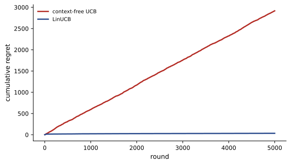
Because no single arm is best for every context, the context-free algorithm, however well it explores, keeps losing reward whenever its favourite arm is wrong for the current user, and its regret grows linearly. LinUCB learns the reward model for each arm and its regret flattens after a short learning period.

Off-policy evaluation

Before deploying a new recommendation or pricing policy, a company wants to know whether it will perform better than the current one. Running an online experiment is the most reliable answer but is slow, costly and risky. Off-policy evaluation estimates a new (target) policy's value from data logged under the old (logging) policy, provided the logs record the probability with which each action was chosen.

Each logged record contains a context \(x_i\), the action taken \(a_i\), the reward \(r_i\), and the propensity \(\mu(a_i \mid x_i)\) under the logging policy. Estimators include:

• Inverse propensity scoring (IPS): reweight each logged reward by how much more (or less) likely the target policy \(\pi\) is to take that action, \(\hat V_{\text{IPS}} = \frac1n\sum_i \frac{\pi(a_i \mid x_i)}{\mu(a_i \mid x_i)}r_i\). It is unbiased if the logging policy gives every action the target might take a non-zero probability, but its variance is large when weights are large.
• Self-normalized IPS: divide by the sum of the weights instead of \(n\), trading a small bias for much lower variance.
• The direct method: fit a reward model \(\hat r(x, a)\) and average its predictions under the target policy. Low variance, but biased if the model is wrong.
• Doubly robust estimation: start from the direct method and correct it with importance-weighted residuals, \(\hat V_{\text{DR}} = \frac1n\sum_i \left[\sum_a \pi(a \mid x_i)\hat r(x_i, a) + \frac{\pi(a_i \mid x_i)}{\mu(a_i \mid x_i)}(r_i - \hat r(x_i, a_i))\right]\). It is unbiased if either the propensities or the reward model are correct, and usually has lower variance than IPS.

import numpy as np

rng = np.random.default_rng(2)
n, K = 20000, 3
x = rng.integers(0, 2, n)                              # one binary context (e.g. new vs returning user)
true_mean = np.array([[0.10, 0.05, 0.08], [0.04, 0.12, 0.06]])   # click rate by context and action
logging = np.array([[0.6, 0.2, 0.2], [0.6, 0.2, 0.2]])           # the old policy mostly shows action 0
a = np.array([rng.choice(K, p=logging[c]) for c in x])
r = (rng.random(n) < true_mean[x, a]).astype(float)

target = np.array([[1.0, 0.0, 0.0], [0.0, 1.0, 0.0]])            # new policy: action 0 for new users, 1 for returning
true_value = np.mean([true_mean[c] @ target[c] for c in (0, 1)])

w = target[x, a] / logging[x, a]                       # importance weights
ips = np.mean(w * r)
snips = np.sum(w * r) / np.sum(w)
# Doubly robust: a reward model (here, empirical means by context and action) plus a weighted correction
model = np.array([[r[(x == c) & (a == k)].mean() for k in range(K)] for c in (0, 1)])
dm = np.mean([model[c] @ target[c] for c in x])
dr = dm + np.mean(w * (r - model[x, a]))
print(f"true value of the new policy {true_value:.4f}; logged policy value {r.mean():.4f}")
print(f"inverse propensity scoring {ips:.4f}; self-normalized {snips:.4f}; direct method {dm:.4f}; doubly robust {dr:.4f}")

true value of the new policy 0.1100; logged policy value 0.0750
inverse propensity scoring 0.1144; self-normalized 0.1128; direct method 0.1127; doubly robust 0.1127

All four estimates are close to the true value of 0.110, showing that the new policy would raise the click rate from 0.075 by nearly half, without running it. This works because the logging policy explored: it showed every action with probability at least 0.2. A logging policy that never showed an action in some context makes the target policy's value in that context impossible to estimate from the logs, whatever the estimator. This is a strong argument for building a little randomization into production systems and always recording propensities.

Bandits in practice

• Bandits versus A/B tests: a classic A/B test splits traffic evenly for a fixed period to estimate the difference between variants with known statistical power, then picks the winner. A bandit shifts traffic toward better variants during the test, reducing the cost of showing poor variants but complicating statistical inference. A/B tests suit decisions that need a clear, defensible estimate; bandits suit continuous optimization among many options.
• Delayed feedback: rewards such as purchases or subscription renewals arrive hours or weeks after the action, so algorithms must update in batches and account for pending outcomes.
• Guardrails: production systems constrain exploration to avoid harmful actions, cap how much traffic a new arm can receive, and monitor secondary metrics such as complaints or long-term retention.
• Feedback loops: a recommender that only learns from what it shows can narrow what users see; exploration and diversity constraints counter this.
• Ethics: in clinical trials, adaptive designs that assign more patients to better treatments raise both benefits and questions of fairness and informed consent, and are regulated accordingly.

When actions change the future context (a recommendation affects what a user wants next, a price affects future demand), the problem stops being a bandit and becomes a full reinforcement learning problem, the subject of the rest of the course.