Reinforcement learning for language models, safety and a project

Lesson 9 introduced reinforcement learning from human feedback, the method that turned pre-trained language models into helpful assistants. Since then, reinforcement learning has become a central part of how large language models are trained: to follow instructions, to refuse harmful requests, and, increasingly, to reason through mathematics and code problems using rewards that can be checked automatically. This final lesson examines the RL objective used for language models and its closed-form solution, direct preference optimization, reward model over-optimization, group-relative policy optimization and RL with verifiable rewards, and the safety questions these raise. It ends with a project applying the course's methods to a real control problem.

The language model as a policy

For RL purposes, a language model is a policy \(\pi_\theta(y \mid x)\) that, given a prompt \(x\), generates a response \(y\) one token at a time. Each token is an action, the prompt and tokens so far form the state, and the episode ends with the response. Rewards usually arrive only at the end, from a reward model, a human rating, or an automatic check such as running unit tests or comparing a final answer with a known solution. The action space (a vocabulary of 50,000 to 200,000 tokens) is huge, but the pre-trained model already places most of its probability on sensible continuations, so RL refines an excellent starting policy rather than learning from scratch.

The KL-regularized objective

RLHF maximizes reward while penalizing divergence from a reference policy \(\pi_{\text{ref}}\), usually the supervised fine-tuned model:

The KL term keeps the policy close to the fluent, broadly capable reference, and limits how far it can move to exploit errors in the reward model. This objective has a closed-form optimum, found by the same reasoning as in maximum entropy RL:

The optimal policy reweights the reference by the exponential of the reward. Small \(\beta\) concentrates probability on the highest-reward responses; large \(\beta\) stays near the reference. In practice the optimum cannot be computed directly, because \(Z(x)\) sums over all possible responses, so it is approached with policy gradient methods such as PPO (Lesson 9), with the KL penalty included in the reward.

Reward model over-optimization

A learned reward model is only an approximation of human preferences, trained on limited comparisons. Optimizing it hard finds the responses it overrates: overly long answers, confident-sounding but wrong claims, flattery, or exploitation of quirks in its training data. Measured against true human judgement, quality first rises with optimization and then falls, a direct instance of Goodhart's law and reward hacking (Lesson 4). Studies of this effect found that the gap between proxy and true reward grows predictably with the KL divergence from the reference.

import numpy as np

rng = np.random.default_rng(13)
n = 2000                                              # possible responses to one prompt
ref = rng.dirichlet(np.ones(n) * 0.5)                 # reference (pre-trained) policy probabilities
true_r = rng.normal(0, 1, n)                          # what humans actually prefer
flawed = rng.random(n) < 0.01                       # 1% of responses exploit a flaw in the reward model:
true_r[flawed] = rng.normal(-1.0, 0.5, flawed.sum())  # people dislike them,
proxy = true_r.copy(); proxy[flawed] += 4.0           # but the reward model scores them highly

for beta in (10.0, 1.0, 0.3, 0.1, 0.03):
    logits = np.log(ref) + proxy / beta               # optimum of E[r] - beta * KL(pi || ref): pi ~ ref * exp(r / beta)
    pi = np.exp(logits - logits.max()); pi /= pi.sum()
    kl = np.sum(pi * np.log(pi / ref))
    print(f"beta {beta:5.2f}: KL from reference {kl:5.2f} nats; proxy reward {pi @ proxy:+.2f}; true reward {pi @ true_r:+.2f}")
print(f"reference policy: proxy {ref @ proxy:+.2f}, true {ref @ true_r:+.2f}")

beta 10.00: KL from reference  0.01 nats; proxy reward +0.14; true reward +0.07
beta  1.00: KL from reference  0.68 nats; proxy reward +1.33; true reward +0.77
beta  0.30: KL from reference  4.11 nats; proxy reward +3.20; true reward +0.03
beta  0.10: KL from reference  9.06 nats; proxy reward +3.99; true reward -0.00
beta  0.03: KL from reference 11.17 nats; proxy reward +4.17; true reward +0.17
reference policy: proxy +0.02, true -0.03

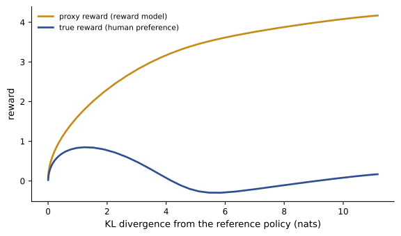
Moderate optimization (\(\beta = 1\)) raises true quality substantially. Pushing further multiplies the proxy reward but sends the true reward back to zero, as the policy concentrates on the flawed responses that the reward model overrates. Mitigations include choosing \(\beta\) and stopping points using held-out human evaluation, ensembles of reward models (optimizing a conservative combination), improving reward models with adversarially collected data, constraining length and style, and auditing samples during training.

Direct preference optimization

Rearranging the closed-form optimum expresses the reward in terms of the optimal policy: \(r(x, y) = \beta\log\frac{\pi^*(y \mid x)}{\pi_{\text{ref}}(y \mid x)} + \beta\log Z(x)\). Substituting this into the Bradley-Terry preference model used to train reward models (Lesson 9), the intractable \(Z(x)\) cancels, because preferences depend only on reward differences between two responses to the same prompt. The result is direct preference optimization (DPO), which trains the policy directly on preference pairs \((y_w, y_l)\) (preferred and dispreferred) with a simple classification loss:

DPO needs no separate reward model and no sampling during training, which makes it simpler and cheaper than PPO-based RLHF. It is an offline method (Lesson 10): it learns only from the fixed preference data set, so it cannot discover and correct the policy's own new failure modes the way online RL can, and it can over-fit to the data. Online and iterative variants, which generate new responses, collect fresh preferences and repeat, combine its simplicity with some of the benefits of on-policy learning.

RL with verifiable rewards and GRPO

For tasks with checkable answers, such as mathematics problems with known solutions, code with unit tests, or formal proofs, the reward can be computed exactly: 1 if the final answer is correct, 0 otherwise. RL with verifiable rewards avoids the reward model and much of its exploitability (though checkers have their own loopholes, such as tests that can be gamed). Trained this way, models learn to produce long chains of reasoning, check intermediate results, and backtrack from mistakes, behaviours that emerged without being explicitly demonstrated.

Group relative policy optimization (GRPO), introduced with the DeepSeekMath models, is a popular algorithm for this setting. For each prompt it samples a group of \(G\) responses, scores them, and uses each response's reward relative to its group as the advantage:

The group mean replaces the learned value function of PPO as the baseline (Lesson 9), saving the memory and computation of a separate critic network the size of the policy, and the update otherwise follows PPO's clipped objective with a KL penalty. Prompts where every response is right or every response is wrong give zero advantage and no learning signal, so training data are often filtered toward problems of intermediate difficulty for the current model.

import numpy as np

rng = np.random.default_rng(14)
# A toy "reasoning" policy chooses one of 4 strategies for each problem; each strategy solves a problem with
# a different probability, and the reward is 1 if the final answer is verified correct.
p_correct = np.array([0.2, 0.35, 0.5, 0.8])
theta = np.array([1.5, 1.0, 0.5, 0.0])                # initial preferences favour the weakest strategy
G, lr = 8, 0.5                                        # group size and learning rate
for step in range(201):
    pi = np.exp(theta - theta.max()); pi /= pi.sum()
    if step % 50 == 0:
        print(f"step {step:3d}: strategy probabilities {np.round(pi, 2)}; expected accuracy {pi @ p_correct:.2f}")
    grad = np.zeros(4)
    for _ in range(16):                               # 16 prompts per step
        acts = rng.choice(4, G, p=pi)
        rewards = (rng.random(G) < p_correct[acts]).astype(float)
        if rewards.std() == 0: continue               # all right or all wrong: no learning signal
        adv = (rewards - rewards.mean()) / rewards.std()   # group-relative advantage, no value network
        for a, A in zip(acts, adv):
            g = -pi.copy(); g[a] += 1                 # gradient of log pi(a) for a softmax policy
            grad += A * g / G
    theta += lr * grad / 16

step   0: strategy probabilities [0.46 0.28 0.17 0.1 ]; expected accuracy 0.35
step  50: strategy probabilities [0.02 0.02 0.04 0.92]; expected accuracy 0.77
step 100: strategy probabilities [0.01 0.01 0.01 0.97]; expected accuracy 0.79
step 150: strategy probabilities [0.   0.01 0.01 0.98]; expected accuracy 0.79
step 200: strategy probabilities [0.   0.   0.01 0.99]; expected accuracy 0.79

Starting from a policy that prefers its weakest strategy, the group-relative updates shift probability to the strategy that succeeds most often, and expected accuracy rises from 0.35 to near the best achievable 0.80 within about 50 steps. No value network is needed: comparing responses within each group provides the baseline.

Process reward models offer a complement to outcome rewards: instead of scoring only the final answer, they score each reasoning step, giving denser feedback and helping identify where reasoning goes wrong, at the cost of needing step-level labels or automated step verification.

Safety and responsible use of RL

Reinforcement learning optimizes objectives with persistence and creativity, which is both its power and its risk. Issues to manage in any deployment include:

• Specification: the reward may not capture what is wanted (reward hacking, Lesson 4); test what the trained policy actually does, not just its reward.
• Distribution shift: policies can behave unpredictably in situations unlike training; keep fallback controllers and monitor inputs.
• Safe exploration: in physical systems, constrain actions during learning (constrained MDPs, shields) and train in simulation first.
• Goal misgeneralization: a policy can learn a goal that coincides with the intended one in training but differs elsewhere, such as following a visual cue that happened to mark the goal.
• Oversight: for powerful systems, human review, interpretability tools and evaluations for dangerous capabilities complement reward-based training. Methods that use AI feedback guided by written principles, such as constitutional AI, scale oversight beyond what human labelling alone allows.

Capstone project: RL for data centre cooling control

The project applies the course to an industrial problem. A data centre wants an RL controller to adjust chilled-water set points, fan speeds and the number of running chillers and cooling towers every five minutes, minimizing energy while keeping server inlet temperatures within limits (DCE-330). Published work on data centre cooling has reported energy savings for cooling on the order of tens of percent with learned controllers operating under safety constraints and human supervision.

Step 1: Formulate the problem

State: outdoor temperature and humidity, IT load, current set points and equipment status, temperatures at key sensors, and recent trends (to make the state closer to Markov, Lesson 4). Actions: set point changes within small allowed steps, and equipment staging. Reward: negative energy use. Constraints: inlet temperatures below limits and minimum run times for equipment, handled as a constrained MDP with a Lagrangian rather than a fixed penalty. Discount: with decisions every 5 minutes and thermal effects over about an hour, a horizon of about 12 to 24 steps suggests \(\gamma \approx 0.95\).

Step 2: Start from data

Years of operating logs from the building management system are available. Use them to train a dynamics model (an ensemble, Lesson 10) predicting temperatures and power from state and action, and evaluate it on held-out periods, checking its accuracy over multi-step rollouts.

Step 3: Learn offline, conservatively

Train a policy offline with a conservative method (CQL or a model-based method with uncertainty penalties), so it does not rely on actions the logs never contain. Evaluate candidate policies with fitted Q evaluation and with the model, and compare with the existing rule-based controller.

Step 4: Deploy safely

Deploy in recommendation mode first, with operators approving each action; then in closed loop with a safety layer that verifies every proposed action against the model and hard limits, reverting to the existing controller if predictions and measurements diverge or any limit is approached. Use model predictive control (Lesson 10) as a planning layer, with the learned value function at the horizon.

Step 5: Improve online

With safety established, allow limited exploration within constraints, update the model and policy periodically, and monitor energy savings, constraint violations and operator overrides. Re-check for distribution shift when IT load patterns change, such as when AI training clusters are added.

The project draws on bandits and evaluation, MDP formulation and constraints, dynamic programming and TD learning, planning, deep and distributional value learning, policy optimization, model-based and offline RL, and safe deployment, which together form the practical toolkit of reinforcement learning.