
AI-320 · Lesson 8 of 12 · 31 min
Bayesian regression and generalized linear models
Regression, predicting an outcome from inputs, is the most common modelling task in practice, and the probabilistic view of it pays off immediately. Treating the coefficients as uncertain gives predictions with honest error bars, regularization falls out of the prior, and the same framework extends from continuous outcomes to binary outcomes, counts and positive quantities by changing the likelihood. This lesson develops Bayesian linear regression in closed form, generalizes to the family of generalized linear models (GLMs), treats Bayesian logistic regression with the Laplace approximation, handles overdispersed and outlier-prone data, and introduces hierarchical regression, the workhorse of applied Bayesian statistics.
Bayesian linear regression
The model is \(y_i = \mathbf{w}^\top\boldsymbol\phi(\mathbf{x}_i) + \varepsilon_i\) with \(\varepsilon_i \sim \mathcal{N}(0, \sigma^2)\), where \(\boldsymbol\phi(\mathbf{x})\) is a vector of features (the inputs themselves, a constant 1 for the intercept, polynomials or other basis functions). With a Gaussian prior \(\mathbf{w} \sim \mathcal{N}(\mathbf{0}, \alpha^{-1}\mathbf{I})\) and known noise variance, the posterior is Gaussian, because the log-likelihood and log-prior are both quadratic in \(\mathbf{w}\):
where \(\boldsymbol\Phi\) is the design matrix whose rows are the feature vectors. The posterior precision is the prior precision plus the data precision, the multivariate version of the update in Lesson 1. The posterior mean is the ridge regression estimate with penalty \(\lambda = \alpha\sigma^2\); as \(\alpha \to 0\) it becomes ordinary least squares.
The predictive distribution for a new input averages over the posterior and is also Gaussian:
The predictive variance has two parts: the irreducible noise \(\sigma^2\), and the parameter uncertainty \(\boldsymbol\phi_*^\top\mathbf{S}\boldsymbol\phi_*\), which shrinks as data accumulate and grows for inputs far from the training data.
Worked problem
A slope through the origin
A model \(y = wx + \varepsilon\) has prior \(w \sim \mathcal{N}(0, 1)\) and noise \(\sigma = 1\). Data: \((x, y) = (1, 2), (2, 3), (3, 7)\). Find the posterior of \(w\) and the predictive distribution at \(x = 4\).
Show solution
- \(\sum x^2 = 1 + 4 + 9 = 14\); \(\sum xy = 2 + 6 + 21 = 29\).
- Posterior precision: \(1 + 14 = 15\), so \(S = 0.0667\) and posterior standard deviation 0.258. Mean: \(29/15 = 1.93\).
- Prediction at \(x = 4\): mean \(4 \times 1.93 = 7.73\); variance \(1 + 16 \times 0.0667 = 2.07\), standard deviation 1.44.
Answer: \(w \sim \mathcal{N}(1.93, 0.258^2)\); \(y_* \sim \mathcal{N}(7.73, 1.44^2)\). The least squares slope would be \(29/14 = 2.07\); the prior pulls it slightly toward zero.
import numpy as np

rng = np.random.default_rng(8)
w_true = np.array([1.0, 2.0])                         # intercept and slope
sigma = 0.5                                           # known noise standard deviation
alpha = 1.0                                           # prior precision: w ~ N(0, I / alpha)

def posterior(X, y):
    Phi = np.column_stack([np.ones(len(X)), X])
    S_inv = alpha * np.eye(2) + Phi.T @ Phi / sigma ** 2
    S = np.linalg.inv(S_inv)
    m = S @ Phi.T @ y / sigma ** 2
    return m, S

for n in (2, 10, 100):
    X = rng.uniform(-1, 1, n)
    y = w_true[0] + w_true[1] * X + rng.normal(0, sigma, n)
    m, S = posterior(X, y)
    sd = np.sqrt(np.diag(S))
    phi = np.array([1.0, 3.0])                        # predict at x = 3, outside the data range
    pred_sd = np.sqrt(sigma ** 2 + phi @ S @ phi)
print(f"n = {n:3d}: slope {m[1]:.2f} +/- {sd[1]:.2f}; prediction at x = 3: {phi @ m:.2f} +/- {pred_sd:.2f} (true {w_true @ phi:.2f})")n = 2: slope 1.89 +/- 0.47; prediction at x = 3: 6.21 +/- 1.41 (true 7.00) n = 10: slope 1.73 +/- 0.36; prediction at x = 3: 6.06 +/- 1.28 (true 7.00) n = 100: slope 2.09 +/- 0.09; prediction at x = 3: 7.30 +/- 0.58 (true 7.00)
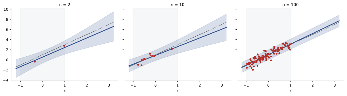
With unknown noise variance, a conjugate normal-inverse-gamma prior keeps the posterior in closed form, and the predictive distribution becomes a Student-t, with heavier tails reflecting the uncertainty in \(\sigma\). The prior precision \(\alpha\) and noise level can also be chosen by maximizing the marginal likelihood, exactly as for Gaussian processes (Lesson 6); Bayesian linear regression with features \(\boldsymbol\phi\) is a GP with kernel \(\alpha^{-1}\boldsymbol\phi(\mathbf{x})^\top\boldsymbol\phi(\mathbf{x}')\).
Generalized linear models
Linear regression assumes a Gaussian outcome whose mean is linear in the inputs. Many outcomes are not Gaussian: whether a customer churns (binary), how many claims a policy generates (a count), how long a repair takes (positive and skewed). A generalized linear model keeps the linear predictor \(\eta = \mathbf{w}^\top\mathbf{x}\) but connects it to the mean of an exponential-family distribution (Lesson 2) through a link function \(g\):
| Outcome | Distribution | Canonical link | Mean as a function of \(\eta\) | Example |
|---|---|---|---|---|
| Continuous | Gaussian | identity | \(\eta\) | house price |
| Binary | Bernoulli | logit \(\log\frac{\mu}{1 - \mu}\) | \(1/(1 + e^{-\eta})\) | churn, default, click |
| Count | Poisson | log | \(e^\eta\) | claims, defects, calls |
| Positive, skewed | Gamma | inverse (log often used) | \(1/\eta\) or \(e^\eta\) | repair time, claim size |
| Category | Categorical | softmax (multinomial logit) | \(e^{\eta_k}/\sum_j e^{\eta_j}\) | product choice |
With the canonical link, the linear predictor is the natural parameter, the log-likelihood is concave in \(\mathbf{w}\) (Lesson 2), and its gradient takes the same simple form for every member: \(\sum_i (y_i - \mu_i)\mathbf{x}_i\). Fitting uses Newton's method, known in this setting as iteratively reweighted least squares (IRLS) because each step solves a weighted least squares problem; it typically converges in a handful of iterations. Standard errors come from the inverse of the Hessian at the optimum.
The coefficients have convenient interpretations. In logistic regression, \(e^{w_j}\) is the odds ratio for a one-unit increase in input \(j\). In Poisson regression with a log link, \(e^{w_j}\) is a rate ratio: the expected count is multiplied by \(e^{w_j}\).
Worked problem
Interpreting a Poisson regression
A Poisson regression of monthly equipment failures has coefficient 0.18 for operating temperature (per 5 °C above 25 °C) and 0.69 for "older model". Exposure differs between sites, so the log of the number of units is included as an offset. Interpret the coefficients.
Show solution
- Temperature: \(e^{0.18} = 1.20\), a 20% higher failure rate for each 5 °C.
- Older model: \(e^{0.69} = 2.0\), twice the failure rate at the same temperature.
- Offset: with \(\log(\text{units})\) entering with a fixed coefficient of 1, the model describes failures per unit, so sites of different sizes are compared fairly.
Answer: Failures per unit rise 20% per 5 °C and double for the older model. Effects multiply: an older unit running 10 °C hot fails at \(2.0 \times 1.2^2 = 2.9\) times the baseline rate.
Bayesian logistic regression
Adding a prior to a GLM makes the posterior non-Gaussian, because the likelihood is no longer quadratic. For logistic regression there is no closed form, but the posterior is usually close to Gaussian, which suggests the Laplace approximation: find the posterior mode \(\mathbf{w}_{\text{MAP}}\) by Newton's method, then approximate the posterior by a Gaussian with covariance equal to the inverse of the negative Hessian at the mode:
The predictive probability averages the sigmoid over this posterior. Plugging in the MAP weights gives overconfident predictions, especially far from the data. The average has no closed form, but the probit approximation is accurate: with predictive mean \(\mu_a = \mathbf{w}_{\text{MAP}}^\top\mathbf{x}_*\) and variance \(\sigma_a^2 = \mathbf{x}_*^\top\mathbf{S}\mathbf{x}_*\),
import numpy as np

rng = np.random.default_rng(9)
n = 30
x = rng.normal(0, 1, n)
p_true = 1 / (1 + np.exp(-(-0.5 + 1.5 * x)))
y = (rng.random(n) < p_true).astype(float)
X = np.column_stack([np.ones(n), x])
prior_prec = 1.0                                      # w ~ N(0, I)

w = np.zeros(2)
for it in range(25):                                  # Newton steps on the log posterior
    p = 1 / (1 + np.exp(-X @ w))
    grad = X.T @ (y - p) - prior_prec * w
    H = -(X.T * (p * (1 - p))) @ X - prior_prec * np.eye(2)
    w = w - np.linalg.solve(H, grad)
S = np.linalg.inv(-H)                                 # Laplace approximation: N(w_map, S)
print(f"MAP weights {np.round(w, 2)}, posterior sd {np.round(np.sqrt(np.diag(S)), 2)}")

for xs in (0.0, 3.0):
    phi = np.array([1.0, xs])
    plug_in = 1 / (1 + np.exp(-phi @ w))
    draws = rng.multivariate_normal(w, S, 20000)      # average the sigmoid over the posterior
    bayes = np.mean(1 / (1 + np.exp(-draws @ phi)))
    mu, var = phi @ w, phi @ S @ phi
    probit = 1 / (1 + np.exp(-mu / np.sqrt(1 + np.pi * var / 8)))
print(f"x = {xs}: plug-in {plug_in:.3f}, Monte Carlo predictive {bayes:.3f}, probit approximation {probit:.3f}")MAP weights [-0.35 1. ], posterior sd [0.38 0.41] x = 0.0: plug-in 0.412, Monte Carlo predictive 0.415, probit approximation 0.415 x = 3.0: plug-in 0.933, Monte Carlo predictive 0.892, probit approximation 0.890
Near the centre of the data the plug-in and Bayesian probabilities agree. At \(x = 3\), where the posterior uncertainty in the slope matters, averaging moderates the prediction from 0.93 to 0.89. The difference matters for decisions with asymmetric costs and for detecting inputs the model knows little about. With only 30 observations, the MAP slope (1.0) is also shrunk below the true 1.5 by the prior, a reminder that priors have influence when data are scarce.
Priors also solve a practical problem. When a single input perfectly separates the classes (complete separation, common with small samples or rare categories), the maximum likelihood coefficient is infinite and the fitting software either fails or reports enormous standard errors. Any proper prior keeps the estimate finite. Weakly informative priors, such as a Student-t or Gaussian with scale around 2.5 on standardized inputs, are a common default.
For more accuracy than the Laplace approximation, MCMC (Lesson 7, particularly Hamiltonian Monte Carlo) samples the exact posterior, and variational inference (Lesson 9) scales to large data sets.
Overdispersion and robustness
Real data often break the simple likelihoods. Counts frequently vary more than a Poisson allows: the Poisson forces variance to equal the mean, but claim counts, website visits and disease cases typically show variance several times the mean, because of unobserved differences between units. Ignoring overdispersion produces standard errors that are far too small. Remedies include:
- The negative binomial distribution, a Poisson whose rate varies according to a gamma distribution, with variance \(\mu + \mu^2/r\).
- A random effect per unit (an observation-level hierarchical term).
- Zero-inflated models when there are more zeros than either distribution predicts, mixing a point mass at zero with a count distribution.
Continuous data with occasional gross errors are handled with a Student-t likelihood in place of the Gaussian. Its heavier tails let the model treat an outlier as a rare large error rather than bending the whole fit toward it. Because the Student-t is a scale mixture of Gaussians (Lesson 2), it can be fitted by EM (Lesson 5) or MCMC.
Hierarchical regression
Data often come in groups: students in schools, sales in stores, patients in hospitals, sensors on machines. Three ways of modelling grouped data illustrate why hierarchical models are so widely used:
- Complete pooling ignores the groups and fits one regression, missing real differences between them.
- No pooling fits a separate regression for each group, which is noisy for small groups and useless for new ones.
- Partial pooling lets each group have its own coefficients, drawn from a common distribution whose parameters are learned from all groups.
A varying-intercept model, for example, writes \(y_{ij} = \alpha_j + \mathbf{w}^\top\mathbf{x}_{ij} + \varepsilon_{ij}\) with \(\alpha_j \sim \mathcal{N}(\mu_\alpha, \tau^2)\). Each group's intercept is estimated as a compromise between its own data and the population mean, weighted by their precisions, exactly the shrinkage of Lesson 1:
Worked problem
Shrinkage of store effects
Store intercepts vary with \(\tau = 2\) around a population mean of 10 (units per day), and daily noise has \(\sigma = 6\). Store A has 4 days of data averaging 16; store B has 100 days averaging 13. Estimate each store's intercept.
Show solution
- Store A: data precision \(4/36 = 0.111\), prior precision \(1/4 = 0.25\). Weight on data: \(0.111/0.361 = 0.31\). Estimate: \(0.31 \times 16 + 0.69 \times 10 = 11.8\).
- Store B: data precision \(100/36 = 2.78\). Weight: \(2.78/3.03 = 0.92\). Estimate: \(0.92 \times 13 + 0.08 \times 10 = 12.8\).
Answer: Store A is estimated at 11.8 despite its high average, because four days are weak evidence; store B at 12.8, close to its own average. Ranking stores by raw averages would put A first, a judgement the data do not support.
Hierarchical models extend naturally: varying slopes, several grouping levels (students in classes in schools), and group-level predictors. They are typically fitted by MCMC, and their posteriors have a funnel shape (when \(\tau\) is small, the group effects are tightly constrained) that challenges samplers; a non-centred parameterization, writing \(\alpha_j = \mu_\alpha + \tau z_j\) with \(z_j \sim \mathcal{N}(0, 1)\), usually cures it. Probabilistic programming languages (Lesson 10) make writing and fitting such models routine.
Common mistakes
MistakeReporting predictions from the posterior mean without parameter uncertainty.
InsteadUse the predictive distribution, which adds \(\boldsymbol\phi_*^\top\mathbf{S}\boldsymbol\phi_*\) to the noise variance.
MistakeFitting a Poisson model to overdispersed counts.
InsteadCheck the variance-to-mean ratio and use a negative binomial or random effects.
MistakeForgetting the exposure offset in count models.
InsteadInclude \(\log(\text{exposure})\) as an offset so that rates are compared fairly.
MistakeUsing maximum likelihood logistic regression with separated data.
InsteadAdd a weakly informative prior to keep coefficients finite.
MistakeRanking small groups by raw averages.
InsteadUse partial pooling, which shrinks noisy estimates toward the population mean.
Summary and key terms
- Bayesian linear regression has a Gaussian posterior and predictive distribution; the posterior mean is ridge regression.
- Predictive variance combines noise and parameter uncertainty, which grows away from the data.
- GLMs connect a linear predictor to an exponential-family mean through a link; IRLS fits them and coefficients become odds or rate ratios.
- Bayesian logistic regression uses the Laplace approximation, and predictive averaging moderates overconfident probabilities.
- Negative binomial, zero-inflated and Student-t models handle overdispersion, excess zeros and outliers.
- Hierarchical regression partially pools groups, shrinking small-group estimates toward the population.
- Design matrix
- The matrix whose rows are the feature vectors of the observations.
- Predictive distribution
- The distribution of a new outcome, averaging over the posterior.
- Generalized linear model
- A model linking a linear predictor to an exponential-family mean.
- Link function
- The function mapping the mean to the linear predictor.
- IRLS
- Iteratively reweighted least squares, Newton's method for GLMs.
- Offset
- A term with a fixed coefficient of 1, often the log of exposure.
- Laplace approximation
- A Gaussian fitted at the posterior mode using the curvature there.
- Complete separation
- When an input perfectly predicts a binary outcome, making MLE coefficients infinite.
- Negative binomial
- A gamma mixture of Poissons for overdispersed counts.
- Partial pooling
- Estimating group effects as a compromise between group data and the population.
Practice problems
Work each problem on paper first, then reveal the answer to check.
Prior \(w \sim \mathcal{N}(0, 1)\), \(\sigma = 1\), data \((1, 1), (1, 3)\) for \(y = wx\): posterior mean and variance?
Show answer
Precision 3, mean \(4/3 = 1.33\), variance 0.333.
Predictive variance at \(x = 2\) for that model?
Show answer
\(1 + 4 \times 0.333 = 2.33\).
Ridge penalty equivalent to prior precision 2 with \(\sigma^2 = 0.25\)?
Show answer
\(\lambda = 0.5\).
Logistic coefficient 0.4: odds ratio?
Show answer
\(e^{0.4} = 1.49\).
Poisson coefficient −0.22 for a training program: effect on the rate?
Show answer
Multiplied by 0.80, a 20% reduction.
Probit approximation with \(\mu_a = 2\) and \(\sigma_a^2 = 4\)?
Show answer
\(\sigma(2/\sqrt{1 + 1.571}) = \sigma(1.25) = 0.78\).
Why does complete separation break maximum likelihood logistic regression?
Show answer
The likelihood keeps increasing as the coefficient grows without bound.
Variance of a negative binomial with mean 10 and \(r = 5\)?
Show answer
\(10 + 100/5 = 30\).
Group with 9 observations, \(\sigma = 3\), \(\tau = 1\): weight on the group mean?
Show answer
\(1/(1 + 1) = 0.5\).
What does a non-centred parameterization fix?
Show answer
The funnel geometry that slows MCMC in hierarchical models.
Lesson quiz · 5 questions
Score 60% or more to complete this lesson.
Create a free account to save your progress, take quizzes and earn a certificate.