Monte Carlo sampling

Almost every quantity of interest in Bayesian inference is an expectation under the posterior: the posterior mean is \(\mathbb E[\theta \mid D]\), a predictive probability is \(\mathbb E[p(\tilde x \mid \theta)]\), a credible interval comes from posterior quantiles, and the probability that B beats A is \(\mathbb E[\mathbf 1(p_B > p_A)]\). Lessons 1 and 3 computed these exactly for conjugate models and small discrete networks. Realistic models have posteriors with no closed form, over thousands or millions of dimensions, where exact integration is impossible. Monte Carlo methods replace integrals by averages over random samples. This lesson covers basic Monte Carlo estimation, direct sampling methods, importance sampling, Markov chain Monte Carlo (MCMC) with the Metropolis-Hastings and Gibbs algorithms, convergence diagnostics, and Hamiltonian Monte Carlo, the engine of modern probabilistic programming.

Monte Carlo estimation

If \(x^{(1)}, \ldots, x^{(S)}\) are independent samples from \(p(x)\), then for any function \(f\)

The estimate is unbiased, and by the central limit theorem its standard error is \(\sigma_f/\sqrt S\), where \(\sigma_f\) is the standard deviation of \(f(x)\). Two facts make Monte Carlo powerful: the error does not depend on the dimension of \(x\), unlike grid-based numerical integration, whose cost grows exponentially with dimension; and the error can be estimated from the samples themselves. The price is slow convergence: each extra decimal digit of accuracy costs 100 times as many samples.

import numpy as np

rng = np.random.default_rng(0)
for S in [100, 10_000, 1_000_000]:
    pts = rng.uniform(-1, 1, size=(S, 2))
    inside = (pts ** 2).sum(axis=1) <= 1
    est = 4 * inside.mean()
    se = 4 * inside.std(ddof=1) / np.sqrt(S)
    print(f"S = {S:>9,}:  pi estimate {est:.5f}  standard error {se:.5f}  actual error {abs(est - np.pi):.5f}")

# the same estimator in 20 dimensions: fraction of the cube inside the unit ball
d, S = 20, 1_000_000
pts = rng.uniform(-1, 1, size=(S, d))
print(f"fraction of 20-D cube inside the ball: {np.mean((pts ** 2).sum(axis=1) <= 1):.2e}  (exact 2.46e-08)")

S =       100:  pi estimate 2.92000  standard error 0.17848  actual error 0.22159
S =    10,000:  pi estimate 3.16360  standard error 0.01627  actual error 0.02201
S = 1,000,000:  pi estimate 3.14152  standard error 0.00164  actual error 0.00007
fraction of 20-D cube inside the ball: 0.00e+00  (exact 2.46e-08)

The standard error shrinks by a factor of 10 for every 100-fold increase in samples, and it correctly predicts the typical size of the actual error. The second experiment shows the catch: the error is independent of dimension only relative to the standard deviation of \(f\). In 20 dimensions, the unit ball fills only \(2.5 \times 10^{-8}\) of the cube, so not one of a million uniform samples lands inside it and the estimate is exactly zero. Sampling from the wrong distribution wastes nearly all samples, which is why the rest of this lesson is about drawing samples from the distribution that matters.

Sampling from simple distributions

Inverse transform sampling

If \(u\) is uniform on (0, 1) and \(F\) is a cumulative distribution function, then \(x = F^{-1}(u)\) has distribution \(F\). For the exponential distribution with rate \(\lambda\), \(F(x) = 1 - e^{-\lambda x}\), so \(x = -\log(1 - u)/\lambda\). Inverse transforms are exact and efficient when \(F^{-1}\) is available; standard libraries use them, along with specialized transformations such as the Box-Muller method for normal variables, to sample all the common distributions.

Rejection sampling

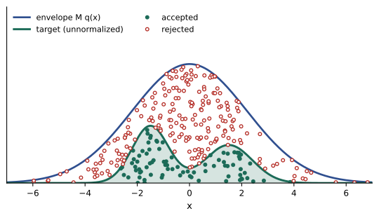
To sample from a density \(p(x) = \tilde p(x)/Z\) known only up to its normalizing constant, choose a proposal \(q(x)\) that is easy to sample and a constant \(M\) with \(\tilde p(x) \le Mq(x)\) everywhere. Draw \(x \sim q\) and \(u \sim U(0, 1)\), and accept \(x\) if \(u < \tilde p(x)/(Mq(x))\). Accepted samples are exact draws from \(p\). The acceptance rate is \(Z/M\), so rejection sampling works only when \(q\) matches \(p\) closely. In high dimensions even small mismatches compound across dimensions, \(M\) becomes astronomically large, and almost every proposal is rejected.

Importance sampling

Instead of rejecting samples, importance sampling keeps them all and weights them. For samples \(x^{(s)} \sim q\),

If \(p\) is known only up to a constant, the self-normalized estimator divides by \(\sum_s w_s\) instead of \(S\). Importance sampling is valuable for rare events, where a good proposal places samples in the important region, and for reweighting samples from one distribution to answer questions about another, as in off-policy evaluation in reinforcement learning. Its weakness is weight degeneracy: if \(q\) has lighter tails than \(p\) or is poorly matched, a few samples carry nearly all the weight and the estimate is unreliable. The effective sample size, \(\mathrm{ESS} = (\sum w_s)^2/\sum w_s^2\), measures how many equally weighted samples the weighted set is worth.

import numpy as np
from scipy.stats import norm

rng = np.random.default_rng(1)
S = 10_000
exact = norm.sf(4.5)                                     # P(X > 4.5) for X ~ N(0, 1)

x = rng.normal(size=S)                                   # naive Monte Carlo
naive = np.mean(x > 4.5)

y = rng.normal(loc=4.5, size=S)                          # proposal centred on the rare region
w = norm.pdf(y) / norm.pdf(y, loc=4.5)
vals = w * (y > 4.5)
imp = vals.mean()
se = vals.std(ddof=1) / np.sqrt(S)
ess = w.sum() ** 2 / (w ** 2).sum()

print(f"exact               {exact:.3e}")
print(f"naive MC            {naive:.3e}  (number of hits: {int(np.sum(x > 4.5))})")
print(f"importance sampling {imp:.3e}  +/- {se:.1e}")
print(f"ESS of the weights for estimating the whole distribution: {ess:.1f} of {S}")

exact               3.398e-06
naive MC            0.000e+00  (number of hits: 0)
importance sampling 3.464e-06  +/- 7.8e-08
ESS of the weights for estimating the whole distribution: 8.5 of 10000

Naive Monte Carlo with 10,000 samples almost never sees an event with probability \(3.4 \times 10^{-6}\), while importance sampling with a shifted proposal estimates it to within about 2%, consistent with its reported standard error. The tiny ESS shows the other side: the same weighted samples would be useless for estimating anything about the bulk of \(p\). A proposal must be matched to the question being asked.

Markov chain Monte Carlo

Rejection and importance sampling need a proposal that already resembles the target, which is impractical for complex posteriors in many dimensions. MCMC takes a different approach: it constructs a Markov chain that wanders through the parameter space and whose long-run distribution of states is the target \(p(x)\). Each state depends on the previous one, so the samples are correlated, but averages over a long run still converge to expectations under \(p\).

A Markov chain with transition kernel \(T(x' \mid x)\) leaves \(p\) invariant if \(\int T(x' \mid x)\,p(x)\,dx = p(x')\). A simple sufficient condition is detailed balance:

meaning that, at equilibrium, the flow of probability from \(x\) to \(x'\) equals the flow back. If the chain also can reach every region (irreducibility) and does not cycle periodically, it converges to \(p\) from any starting point.

Metropolis-Hastings

The Metropolis-Hastings algorithm builds such a chain from any proposal distribution \(q(x' \mid x)\). From the current state \(x\), propose \(x' \sim q(x' \mid x)\) and accept it with probability

otherwise stay at \(x\) (and count \(x\) again as the next sample). Only the ratio \(\tilde p(x')/\tilde p(x)\) is needed, so the normalizing constant, which is the hard part of Bayesian inference, cancels. With a symmetric proposal such as a Gaussian random walk, \(q\) cancels too, giving the original Metropolis algorithm: always move uphill, and move downhill with probability equal to the density ratio.

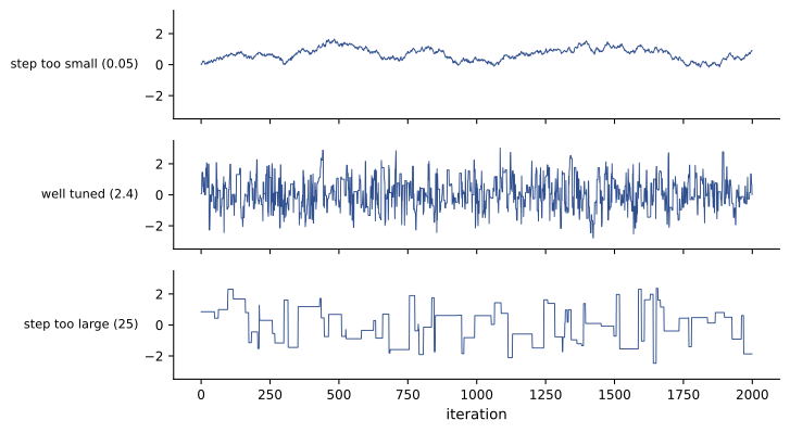
The proposal scale controls efficiency. Tiny steps are almost always accepted but explore slowly, like a random walk with short strides; huge steps propose distant points that are almost always rejected, so the chain sits still. For random-walk Metropolis in high dimensions, theory suggests tuning the scale for an acceptance rate around 23%, and around 44% in one dimension.

import numpy as np

def log_target(x):                       # correlated 2-D Gaussian, correlation 0.9
    P = np.linalg.inv(np.array([[1.0, 0.9], [0.9, 1.0]]))
    return -0.5 * x @ P @ x

def ess(chain):                          # effective sample size from autocorrelations
    x = chain - chain.mean(); n = len(x)
    acf = np.correlate(x, x, mode="full")[n - 1:] / (x @ x)
    s = 0.0
    for k in range(1, n // 2, 2):        # sum pairs while positive (Geyer)
        pair = acf[k] + acf[k + 1]
        if pair < 0: break
        s += pair
    return n / (1 + 2 * s)

rng = np.random.default_rng(2)
for step in [0.05, 0.5, 1.2, 5.0]:
    x = np.zeros(2); lp = log_target(x); chain = []; acc = 0
    for _ in range(20_000):
        prop = x + step * rng.normal(size=2)
        lp_prop = log_target(prop)
        if np.log(rng.uniform()) < lp_prop - lp:
            x, lp = prop, lp_prop; acc += 1
        chain.append(x[0])
    chain = np.array(chain[2000:])
    print(f"step {step:4.2f}: acceptance {acc / 20_000:5.1%}  mean {chain.mean():+.3f}  "
          f"var {chain.var():.3f}  ESS {ess(chain):7.0f} of {len(chain)}")

step 0.05: acceptance 94.7%  mean -0.109  var 0.709  ESS       5 of 18000
step 0.50: acceptance 53.9%  mean -0.042  var 0.998  ESS     273 of 18000
step 1.20: acceptance 25.8%  mean -0.019  var 0.964  ESS     823 of 18000
step 5.00: acceptance  3.4%  mean -0.020  var 1.025  ESS     229 of 18000

The true mean is 0 and the variance is 1. The smallest step accepts almost every proposal but moves so little that 18,000 samples are worth only a handful of independent ones, and its estimates are poor. The largest step rejects nearly everything. The intermediate scales, with acceptance rates of about 25 to 55%, give far more effective samples, and the best of the four, at 26% acceptance, is close to the theoretical optimum. Even the best scale yields an ESS far below the chain length, because the strong correlation forces small steps along the narrow direction; this is the motivation for the gradient-based methods below.

Gibbs sampling

Gibbs sampling updates one variable (or block of variables) at a time by sampling it from its full conditional distribution given all the others, \(x_i \sim p(x_i \mid \mathbf x_{-i})\). It is a special case of Metropolis-Hastings whose acceptance probability is always 1. In a graphical model, the full conditional depends only on the variable's Markov blanket (Lesson 3), and in conjugate models it often has a standard form, so Gibbs sampling needs no tuning. It was the workhorse of Bayesian computation for decades, through software such as BUGS and JAGS, and is still used for topic models and many hierarchical models.

Its weakness is strongly correlated variables: updating one coordinate at a time with the other held fixed allows only tiny moves along a narrow ridge, so the chain mixes slowly.

import numpy as np

rng = np.random.default_rng(3)
for rho in [0.0, 0.9, 0.99]:
    x = y = 0.0; xs = []
    sd = np.sqrt(1 - rho ** 2)
    for _ in range(20_000):
        x = rng.normal(rho * y, sd)          # x | y ~ N(rho y, 1 - rho^2)
        y = rng.normal(rho * x, sd)          # y | x ~ N(rho x, 1 - rho^2)
        xs.append(x)
    xs = np.array(xs[1000:])
    lag1 = np.corrcoef(xs[:-1], xs[1:])[0, 1]
    print(f"rho = {rho:4.2f}: lag-1 autocorrelation {lag1:.3f}  (theory {rho ** 2:.3f})  "
          f"sample variance {xs.var():.3f}")

rho = 0.00: lag-1 autocorrelation -0.001  (theory 0.000)  sample variance 0.988
rho = 0.90: lag-1 autocorrelation 0.807  (theory 0.810)  sample variance 0.993
rho = 0.99: lag-1 autocorrelation 0.980  (theory 0.980)  sample variance 0.969

For the bivariate normal, the lag-1 autocorrelation of the Gibbs chain is \(\rho^2\). At \(\rho = 0.99\) it is 0.98, so roughly 100 iterations are needed per effectively independent sample. Reparameterizing to reduce posterior correlations, or updating correlated variables together in blocks, are the standard remedies.

Diagnosing convergence

An MCMC run produces numbers whatever happens, so checking that they represent the target is essential. Standard practice:

• Burn-in (warm-up): discard the early part of each chain, before it reaches the high-probability region from its arbitrary starting point. Modern samplers also use warm-up to tune step sizes.
• Trace plots: plot each parameter against iteration. A healthy chain looks like stationary noise ("a fuzzy caterpillar"); trends, long flat stretches or slow wandering indicate problems.
• Multiple chains from dispersed starting points: if they agree, there is some confidence they have found the same distribution. The potential scale reduction factor \(\hat R\) compares the variance between chains with the variance within them; values above about 1.01 signal that the chains have not mixed.
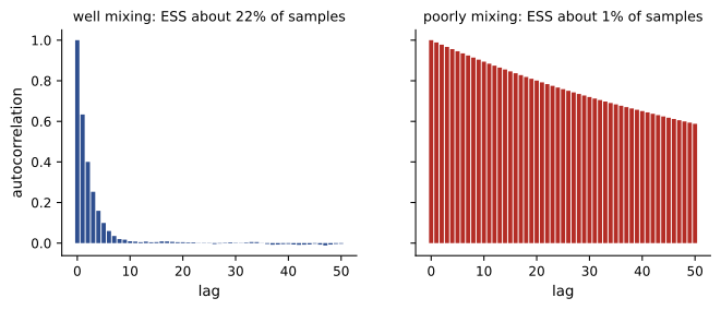
• Effective sample size: because samples are autocorrelated, \(S\) correlated draws carry the information of \(\mathrm{ESS} = S/(1 + 2\sum_k \rho_k)\) independent ones, where \(\rho_k\) is the lag-\(k\) autocorrelation. The Monte Carlo standard error of a posterior mean is \(\sigma/\sqrt{\mathrm{ESS}}\). A few hundred effective samples per quantity is usually enough for means and central intervals; tail quantiles need more.

Diagnostics can show that something is wrong but never prove that a chain has converged: a multimodal posterior can trap every chain in one mode, and all diagnostics then look perfect. Thinning (keeping every \(k\)th sample) saves storage but does not improve estimates.

Hamiltonian Monte Carlo

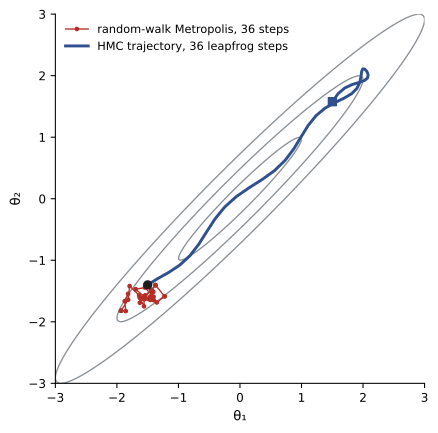
Random-walk proposals explore by diffusion, so the number of steps needed to cross a distribution grows with the square of its width relative to the step size, and in \(d\) dimensions the step size must shrink as dimension grows. Hamiltonian Monte Carlo (HMC) uses the gradient of the log density to make long, directed moves. It introduces an auxiliary momentum variable \(\mathbf r\) and treats \(-\log\tilde p(\mathbf x)\) as a potential energy surface: a frictionless particle with random initial momentum slides across the surface, following Hamilton's equations, and its end point is the proposal.

The dynamics are simulated with the leapfrog integrator for \(L\) steps of size \(\epsilon\), and a Metropolis test corrects for integration error. Because the simulated trajectory nearly conserves \(H\), proposals far from the start are accepted with high probability. HMC scales much better with dimension than random-walk methods and handles correlated posteriors well, especially when the mass matrix \(M\) is adapted to the posterior covariance during warm-up.

The No-U-Turn Sampler (NUTS) chooses the trajectory length automatically by extending it until it starts to double back, and with step-size adaptation it makes HMC essentially tuning-free. NUTS is the default sampler in Stan, PyMC and NumPyro, which let users write a model in a few lines and obtain posterior samples together with diagnostics such as \(\hat R\), ESS and divergent-transition warnings, which flag regions of high curvature where the sampler cannot be trusted. HMC requires continuous parameters and differentiable log densities; discrete latent variables must be summed out or handled with other samplers.

Sequential Monte Carlo

Some problems require updating a posterior repeatedly as data arrive, such as tracking a moving object or estimating a machine's hidden state from streaming sensor data. Particle filters represent the posterior over the current state by a weighted set of samples (particles): each new observation reweights them by its likelihood (importance sampling), and resampling replaces low-weight particles with copies of high-weight ones to avoid degeneracy. Particle filters generalize the HMM forward algorithm of Lesson 3 to continuous and non-linear state spaces, and sequential Monte Carlo methods built on the same ideas also estimate marginal likelihoods.

Lesson 8 applies these samplers to Bayesian regression and hierarchical models, Lesson 10 places them inside probabilistic programming systems and the Bayesian workflow, and Lesson 11 develops particle filters in detail.