
AI-320 · Lesson 2 of 12 · 33 min
Distributions, the exponential family and estimation
Every probabilistic model is assembled from a small set of standard distributions. A mixture model is a categorical choice followed by Gaussians; a topic model is Dirichlets and categoricals; a count regression is a Poisson whose rate depends on inputs. Knowing these building blocks well, and knowing the shared structure most of them have, makes the rest of the course easier: conjugate updates, the EM algorithm, generalized linear models and variational inference all exploit that structure. This lesson reviews the distributions used throughout, the two main ways of estimating their parameters from data (maximum likelihood and maximum a posteriori), the exponential family that unifies them, the multivariate Gaussian and its conditioning rules, and the information-theoretic quantities (entropy and KL divergence) that connect estimation to approximation.
The building blocks
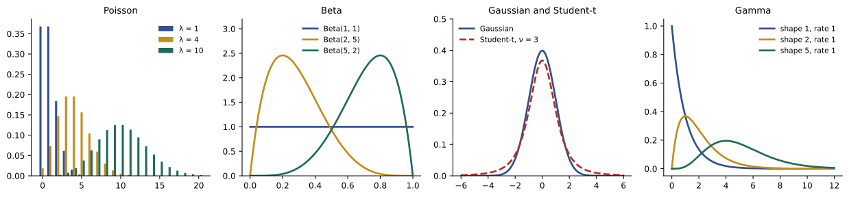
Each distribution suits a type of variable. The table lists the ones used most in this course, with their means and variances.
| Distribution | Support | Parameters | Mean | Variance | Typical use |
|---|---|---|---|---|---|
| Bernoulli | \(\{0, 1\}\) | \(\theta\) | \(\theta\) | \(\theta(1 - \theta)\) | one yes/no outcome |
| Binomial | \(0, \ldots, n\) | \(n, \theta\) | \(n\theta\) | \(n\theta(1 - \theta)\) | successes in \(n\) trials |
| Categorical | \(1, \ldots, K\) | \(\boldsymbol\pi\) | — | — | class labels, words |
| Poisson | \(0, 1, 2, \ldots\) | \(\lambda\) | \(\lambda\) | \(\lambda\) | counts per interval |
| Gaussian | \(\mathbb{R}\) | \(\mu, \sigma^2\) | \(\mu\) | \(\sigma^2\) | measurements, noise |
| Gamma | \((0, \infty)\) | \(a, b\) (shape, rate) | \(a/b\) | \(a/b^2\) | rates, precisions, waiting times |
| Beta | \((0, 1)\) | \(a, b\) | \(a/(a + b)\) | \(\frac{ab}{(a + b)^2(a + b + 1)}\) | probabilities |
| Dirichlet | probability vectors | \(\boldsymbol\alpha\) | \(\alpha_k / \sum_j \alpha_j\) | — | distributions over categories |
| Student-t | \(\mathbb{R}\) | \(\nu, \mu, \sigma\) | \(\mu\) (if \(\nu > 1\)) | larger than Gaussian | robust noise models |
Several relationships connect them. A binomial is a sum of Bernoullis. A Poisson is the limit of a binomial with many trials and small probability. The Beta is the distribution of a probability, and the Dirichlet its multivariate generalization. A Student-t is a Gaussian whose precision is itself gamma-distributed, which gives it heavier tails, so it is used when outliers must not dominate a fit. Choosing a distribution is a modelling decision: counts that vary more than their mean (overdispersion) are poorly fitted by a Poisson, and residuals with occasional large errors are poorly fitted by a Gaussian.
Maximum likelihood estimation
Given data \(x_1, \ldots, x_n\) assumed independent from \(p(x \mid \theta)\), the maximum likelihood estimate (MLE) chooses the parameter that makes the observed data most probable:
Working with the log-likelihood turns products into sums and does not change the maximizer. For many standard distributions the MLE has a closed form found by setting the derivative to zero.
Worked problem
Poisson MLE
A help desk records calls per hour over 6 hours: 2, 4, 3, 5, 1, 3. Find the MLE of the Poisson rate.
Show solution
- Log-likelihood: \(\ell(\lambda) = \sum_i (x_i \log\lambda - \lambda - \log x_i!) = 18\log\lambda - 6\lambda + \text{const}\).
- Derivative: \(18/\lambda - 6 = 0\), so \(\lambda = 3\).
Answer: \(\hat\lambda = 3\) calls per hour, the sample mean. The same pattern (MLE equals a sample average of some statistic) holds for every exponential-family distribution, as shown below.
Maximum likelihood has strong large-sample properties. Under regularity conditions, it is consistent (it converges to the true parameter as \(n\) grows) and asymptotically normal, with variance given by the inverse of the Fisher information:
The Fisher information measures how sharply the log-likelihood curves around its peak: sharper curvature means the data pin the parameter down more precisely. For the Poisson, \(I(\lambda) = 1/\lambda\), so the standard error of \(\hat\lambda\) is \(\sqrt{\lambda/n}\); for the help desk, about \(\sqrt{3/6} = 0.71\) calls per hour.
For small samples, the MLE can behave badly. It can be biased: the MLE of a Gaussian variance divides by \(n\) rather than \(n - 1\) and is too small on average. It can also be extreme: three heads in three coin flips give \(\hat\theta = 1\), a claim that tails are impossible. And in models with many parameters it overfits, which is the reason for the regularization methods of AI-310.
Maximum a posteriori estimation
The maximum a posteriori (MAP) estimate adds a prior and maximizes the posterior density instead (Lesson 1):
The log prior acts as a penalty. With a Gaussian prior \(\theta \sim \mathcal{N}(0, \tau^2)\), the penalty is \(\theta^2/(2\tau^2)\): MAP estimation with a Gaussian prior is exactly L2 regularization (ridge regression, weight decay). A Laplace prior \(p(\theta) \propto e^{-|\theta|/b}\) gives the L1 penalty of the lasso. Regularization, often introduced as an engineering fix, is therefore Bayesian estimation with a particular prior.
MAP is a point estimate, not a posterior. It ignores the posterior's width, and unlike the posterior mean it depends on how the parameter is written (the mode of a density changes under a nonlinear change of variables, such as from \(\sigma\) to \(\log\sigma\)). It is best seen as a cheap approximation, useful when full posterior inference is too costly.
import numpy as np

rng = np.random.default_rng(3)
theta_true = 0.3
a, b = 2.0, 2.0                                   # Beta(2, 2) prior, pulling estimates toward 0.5
for n in (5, 20, 200):
    errs = {"MLE": [], "MAP": [], "posterior mean": []}
    for _ in range(20000):
        k = rng.binomial(n, theta_true)
        errs["MLE"].append(k / n)
        errs["MAP"].append((k + a - 1) / (n + a + b - 2))
        errs["posterior mean"].append((k + a) / (n + a + b))
    row = ", ".join(f"{m} {np.mean((np.array(v) - theta_true) ** 2):.4f}" for m, v in errs.items())
    print(f"n = {n:3d}  mean squared error: {row}")

# The MLE of a Gaussian variance divides by n and is biased low
x = rng.normal(0, 2.0, size=(100000, 5))
v_mle = x.var(axis=1)                             # divides by n
v_unb = x.var(axis=1, ddof=1)                     # divides by n - 1
print(f"true variance 4.00; average MLE {v_mle.mean():.2f}; average unbiased {v_unb.mean():.2f}")n = 5 mean squared error: MLE 0.0420, MAP 0.0247, posterior mean 0.0208 n = 20 mean squared error: MLE 0.0106, MAP 0.0092, posterior mean 0.0086 n = 200 mean squared error: MLE 0.0010, MAP 0.0010, posterior mean 0.0010 true variance 4.00; average MLE 3.21; average unbiased 4.01
With 5 observations, the prior halves the mean squared error, because the MLE's variance is large and the prior pulls extreme estimates back. With 200 observations, the data overwhelm the prior and the three estimates agree. The variance simulation shows the MLE averaging 3.2 instead of 4 with \(n = 5\): its expected value is \((n - 1)/n\) times the true variance.
The exponential family
Most of the distributions in the table belong to one family. A distribution is in the exponential family if its density can be written as
where \(\boldsymbol\eta\) is the natural parameter, \(T(x)\) the sufficient statistic, \(h(x)\) a base measure, and \(A(\boldsymbol\eta)\) the log-partition function that makes the density integrate to one. Examples:
- Bernoulli: \(p(x \mid \theta) = \theta^x(1 - \theta)^{1 - x} = \exp\!\left(x\log\frac{\theta}{1 - \theta} + \log(1 - \theta)\right)\), so \(\eta = \log\frac{\theta}{1 - \theta}\) (the log-odds), \(T(x) = x\), and \(A(\eta) = \log(1 + e^\eta)\).
- Poisson: \(p(x \mid \lambda) = \frac{1}{x!}\exp(x\log\lambda - \lambda)\), so \(\eta = \log\lambda\), \(T(x) = x\), \(A(\eta) = e^\eta\).
- Gaussian: \(\boldsymbol\eta = (\mu/\sigma^2, -1/(2\sigma^2))\) and \(T(x) = (x, x^2)\).
Gamma, beta, Dirichlet, categorical and multivariate Gaussian are also members; Student-t and mixtures are not. Membership brings several properties that the rest of the course uses repeatedly:
- Sufficient statistics. The likelihood of \(n\) observations depends on the data only through \(\sum_i T(x_i)\). For a Poisson, only the total count matters; for a Gaussian, only \(\sum x_i\) and \(\sum x_i^2\). Data can be summarized without loss for estimation, which makes streaming and distributed estimation easy.
- Moments from the log-partition function. The gradient of \(A\) gives the mean of the sufficient statistic, and its second derivative (Hessian) gives the variance: \(\nabla A(\boldsymbol\eta) = \mathbb{E}[T(x)]\) and \(\nabla^2 A(\boldsymbol\eta) = \mathrm{Cov}[T(x)]\). Because a covariance is positive semidefinite, \(A\) is convex, so the log-likelihood is concave in \(\boldsymbol\eta\) and has no spurious local maxima.
- Moment matching. Setting the gradient of the log-likelihood to zero gives \(\nabla A(\hat{\boldsymbol\eta}) = \frac{1}{n}\sum_i T(x_i)\): the MLE is the parameter whose expected sufficient statistics equal the observed averages. This is why the Poisson MLE is the sample mean and the Gaussian MLE uses the sample mean and mean square.
- Conjugate priors. Every exponential-family likelihood has a conjugate prior of the form \(p(\boldsymbol\eta) \propto \exp(\boldsymbol\eta^\top \boldsymbol\chi - \nu A(\boldsymbol\eta))\), and the posterior simply adds the observed sufficient statistics to \(\boldsymbol\chi\) and the count to \(\nu\). The conjugate pairs of Lesson 1 are all instances.
- Generalized linear models. Letting the natural parameter be a linear function of inputs gives logistic regression (Bernoulli), Poisson regression and linear regression (Gaussian) in one framework (Lesson 8).
import numpy as np

# Poisson in exponential-family form: natural parameter eta = log(lambda), A(eta) = exp(eta)
counts = np.array([3, 1, 4, 1, 5, 9, 2, 6, 5, 3])
T = counts.sum()                                  # sufficient statistic: the total is all that matters
n = len(counts)

def loglik(eta):
    return eta * T - n * np.exp(eta)              # dropping the log(x!) terms, which do not involve eta

etas = np.linspace(0.5, 2.0, 15001)
eta_hat = etas[np.argmax(loglik(etas))]
print(f"sufficient statistic T = {T}, n = {n}")
print(f"numerical MLE: lambda = {np.exp(eta_hat):.3f}; closed form T/n = {T / n:.3f}")

# The derivative of the log-partition function gives the mean, the second derivative the variance
h = 1e-4
A = lambda e: np.exp(e)
eta0 = np.log(3.9)
d1 = (A(eta0 + h) - A(eta0 - h)) / (2 * h)
d2 = (A(eta0 + h) - 2 * A(eta0) + A(eta0 - h)) / h ** 2
print(f"at lambda = 3.9: dA/deta = {d1:.3f} (mean), d2A/deta2 = {d2:.3f} (variance)")

# Any data set with the same total gives the same likelihood for lambda
other = np.array([39, 0, 0, 0, 0, 0, 0, 0, 0, 0])
print(f"same T, different data: log-likelihoods equal? {np.isclose(loglik(eta0), eta0 * other.sum() - n * np.exp(eta0))}")sufficient statistic T = 39, n = 10 numerical MLE: lambda = 3.900; closed form T/n = 3.900 at lambda = 3.9: dA/deta = 3.900 (mean), d2A/deta2 = 3.900 (variance) same T, different data: log-likelihoods equal? True
The last line makes the point of sufficiency concrete: a data set with one count of 39 and nine zeros has the same likelihood for \(\lambda\) as the original. The model cannot tell them apart, which is also a warning: if those two data sets should lead to different conclusions (the first is clearly not Poisson), the model is wrong, and only checking the fit (Lesson 10) will reveal it.
The multivariate Gaussian
The multivariate Gaussian is the most important continuous distribution in probabilistic modelling. A vector \(\mathbf{x} \in \mathbb{R}^d\) with mean \(\boldsymbol\mu\) and covariance \(\boldsymbol\Sigma\) has density
Its contours are ellipses whose axes are the eigenvectors of \(\boldsymbol\Sigma\). Two operations keep it Gaussian, and they are the foundation of Gaussian processes (Lesson 6), Bayesian linear regression (Lesson 8) and the Kalman filter (Lesson 11). Partition \(\mathbf{x}\) into \(\mathbf{x}_a\) and \(\mathbf{x}_b\), with blocks of the mean and covariance:
- Marginalizing: \(\mathbf{x}_a \sim \mathcal{N}(\boldsymbol\mu_a, \boldsymbol\Sigma_{aa})\). Just read off the blocks.
- Conditioning: \(\mathbf{x}_a \mid \mathbf{x}_b \sim \mathcal{N}(\boldsymbol\mu_{a|b}, \boldsymbol\Sigma_{a|b})\), with
The conditional mean shifts by an amount proportional to how surprising \(\mathbf{x}_b\) is, and the conditional covariance shrinks by an amount that does not depend on the observed value at all, only on how strongly the variables are correlated.
Worked problem
Conditioning a bivariate Gaussian
Heights of fathers and adult sons (cm) are jointly Gaussian with means 175 and 177, standard deviations 7 and 7, and correlation 0.5. A father is 189 cm tall. What is the distribution of his son's height?
Show solution
- Covariance: \(\Sigma_{ab} = 0.5 \times 7 \times 7 = 24.5\); \(\Sigma_{bb} = 49\).
- Conditional mean: \(177 + (24.5/49)(189 - 175) = 177 + 0.5 \times 14 = 184\) cm.
- Conditional variance: \(49 - 24.5^2/49 = 49 - 12.25 = 36.75\), standard deviation 6.1 cm.
Answer: Gaussian with mean 184 cm and standard deviation 6.1 cm. The son is expected to be tall, but only half as far above average as his father: regression to the mean, which Galton discovered in exactly this setting.
A related fact: a linear function of a Gaussian is Gaussian. If \(\mathbf{x} \sim \mathcal{N}(\boldsymbol\mu, \boldsymbol\Sigma)\), then \(\mathbf{A}\mathbf{x} + \mathbf{b} \sim \mathcal{N}(\mathbf{A}\boldsymbol\mu + \mathbf{b}, \mathbf{A}\boldsymbol\Sigma\mathbf{A}^\top)\). To sample from a multivariate Gaussian, compute a Cholesky factor \(\boldsymbol\Sigma = \mathbf{L}\mathbf{L}^\top\), draw independent standard normals \(\mathbf{z}\), and return \(\boldsymbol\mu + \mathbf{L}\mathbf{z}\), the same reparameterization used in variational inference (Lesson 9).
Entropy, cross-entropy and KL divergence
Information theory supplies the measures used to compare distributions. The entropy of a distribution \(p\) is its average surprise:
A fair coin has entropy \(\log 2\) (one bit, if logs are base 2); a coin that always lands heads has zero entropy. Among all distributions on the real line with a given variance, the Gaussian has the largest entropy, one justification for using it when only the mean and variance are known. More generally, the maximum entropy distribution subject to fixed expectations of some statistics is always an exponential-family distribution with those statistics as \(T(x)\).
The cross-entropy \(H(p, q) = -\sum_x p(x)\log q(x)\) is the average surprise when outcomes follow \(p\) but are coded or predicted with \(q\). The Kullback-Leibler (KL) divergence is the excess:
It is zero only when \(p = q\), and it is not symmetric. These quantities tie the course together:
- Maximizing likelihood is minimizing the KL divergence from the empirical data distribution to the model, because \(\frac1n\sum_i \log q(x_i)\) is the negative cross-entropy of the data under the model, and the data entropy does not depend on the model.
- The cross-entropy loss used to train classifiers is the negative log-likelihood of a categorical model.
- Variational inference minimizes \(\mathrm{KL}(q \,\|\, p)\) from an approximation to the posterior, and the direction matters (Lesson 9).
Worked problem
KL divergence between two coins
A coin truly lands heads with probability 0.5, but a model assigns 0.8. Compute \(\mathrm{KL}(p \,\|\, q)\) and \(\mathrm{KL}(q \,\|\, p)\) in nats.
Show solution
- \(\mathrm{KL}(p \,\|\, q) = 0.5\log(0.5/0.8) + 0.5\log(0.5/0.2) = 0.5(-0.470) + 0.5(0.916) = 0.223\).
- \(\mathrm{KL}(q \,\|\, p) = 0.8\log(0.8/0.5) + 0.2\log(0.2/0.5) = 0.8(0.470) + 0.2(-0.916) = 0.193\).
Answer: 0.223 and 0.193 nats: close but not equal, showing the asymmetry. Each nat of KL per observation is the average log-likelihood ratio by which the data favour the true model, so after about 20 tosses the evidence against the 0.8 model is roughly \(e^{4.5}\), or 90 to 1.
Common mistakes
MistakeUsing a Poisson for counts whose variance far exceeds the mean.
InsteadCheck for overdispersion and use a negative binomial or a hierarchical model.
MistakeTrusting the MLE with very little data.
InsteadUse a prior (MAP or full posterior) or report uncertainty; small-sample MLEs can be biased or extreme.
MistakeTreating MAP as if it were the posterior.
InsteadMAP gives a point; it ignores width and depends on parameterization.
MistakeAssuming KL divergence is a symmetric distance.
Instead\(\mathrm{KL}(p \,\|\, q) \neq \mathrm{KL}(q \,\|\, p)\) in general, and the choice matters.
MistakeForgetting that the conditional covariance of a Gaussian does not depend on the observed value.
InsteadOnly the conditional mean moves; the uncertainty depends on correlations alone.
Summary and key terms
- Standard distributions model binary, categorical, count, continuous and probability-valued variables; choosing one is a modelling decision.
- The MLE maximizes the log-likelihood; it is consistent and asymptotically normal, with variance from the Fisher information, but can misbehave with little data.
- MAP estimation adds a log prior; Gaussian and Laplace priors give L2 and L1 regularization.
- Exponential-family distributions have sufficient statistics, moments from the log-partition function, concave log-likelihoods, moment-matching MLEs and conjugate priors.
- Multivariate Gaussians stay Gaussian under marginalizing, conditioning and linear maps.
- Entropy, cross-entropy and KL divergence connect maximum likelihood, classification losses and variational inference.
- Maximum likelihood estimate
- The parameter maximizing the probability of the observed data.
- Fisher information
- The expected curvature of the log-likelihood; its inverse gives the asymptotic variance of the MLE.
- MAP estimate
- The mode of the posterior distribution.
- Exponential family
- Distributions of the form \(h(x)\exp(\eta^\top T(x) - A(\eta))\).
- Natural parameter
- The parameter \(\eta\) multiplying the sufficient statistic.
- Sufficient statistic
- A function of the data carrying all the information about the parameter.
- Log-partition function
- The normalizer \(A(\eta)\), whose derivatives give the moments.
- Overdispersion
- Count data more variable than a Poisson with the same mean.
- Entropy
- The expected surprise \(-\sum p\log p\) of a distribution.
- KL divergence
- The expected log ratio \(\sum p\log(p/q)\), a non-symmetric measure of difference.
Practice problems
Work each problem on paper first, then reveal the answer to check.
Counts 0, 2, 1, 3, 4: Poisson MLE?
Show answer
2.
Standard error of that estimate (using \(\sqrt{\lambda/n}\))?
Show answer
\(\sqrt{2/5} = 0.63\).
7 successes in 10 trials with a Beta(2, 2) prior: MLE, MAP and posterior mean?
Show answer
0.70, 8/12 = 0.667, 9/14 = 0.643.
What prior corresponds to L2 regularization?
Show answer
A zero-mean Gaussian.
Natural parameter of a Bernoulli with \(\theta = 0.8\)?
Show answer
\(\log 4 = 1.39\).
Sufficient statistics of a Gaussian with unknown mean and variance?
Show answer
\(\sum x_i\) and \(\sum x_i^2\) (with \(n\)).
Why is the exponential-family log-likelihood concave in \(\eta\)?
Show answer
Its Hessian is minus a covariance matrix.
Bivariate Gaussian with standard deviations 2 and 4, correlation 0.6: conditional standard deviation of the second given the first?
Show answer
\(4\sqrt{1 - 0.36} = 3.2\).
Entropy of a fair six-sided die in bits?
Show answer
\(\log_2 6 = 2.58\).
Maximizing likelihood minimizes which KL divergence?
Show answer
From the empirical data distribution to the model, KL(data ‖ model).
Lesson quiz · 5 questions
Score 60% or more to complete this lesson.
Create a free account to save your progress, take quizzes and earn a certificate.