
AI-320 · Lesson 1 of 12 · 34 min
Bayesian reasoning
Most of machine learning, as taught in earlier courses, produces a single answer: one set of weights, one prediction, one cluster label. But data are always finite and noisy, so many answers are consistent with them. Probabilistic modelling keeps track of that uncertainty explicitly. It describes how the data could have been generated, treats the unknown quantities as random variables, and uses the rules of probability to work out what the observed data say about them. The result is not a single answer but a distribution over answers, which tells us how confident to be, how to combine evidence from different sources, and how to make decisions when being wrong has costs.
This course develops that toolkit. This lesson sets out Bayesian reasoning: Bayes' theorem, priors and posteriors, conjugate models, prediction, decisions and model comparison. Later lessons build the standard distributions and estimation methods, graphical models, latent variables, Gaussian processes, Monte Carlo sampling, Bayesian regression, variational inference, model checking, state-space models and uncertainty in machine learning; the section at the end of this lesson shows how they fit together. The course assumes the probability and statistics of STAT-252 and the machine learning foundations of AI-210.
Bayes' theorem
For a hypothesis or parameter \(\theta\) and observed data \(D\), the definition of conditional probability gives Bayes' theorem:
Each term has a name. The prior \(p(\theta)\) expresses what is believed about \(\theta\) before seeing the data. The likelihood \(p(D \mid \theta)\), viewed as a function of \(\theta\), measures how well each value explains the data. The posterior \(p(\theta \mid D)\) is the updated belief. The evidence or marginal likelihood \(p(D)\) is the normalizing constant: it does not depend on \(\theta\), so for many purposes we write simply posterior \(\propto\) likelihood \(\times\) prior.
Bayes' theorem is uncontroversial as mathematics; the Bayesian approach is distinctive in applying it to parameters, treating them as uncertain quantities with distributions rather than fixed unknown constants. The frequentist approach of classical statistics instead reasons about the distribution of estimators over hypothetical repeated data sets. Both are used throughout machine learning, and they often agree when data are plentiful; they differ most when data are scarce, when prior knowledge is strong, or when the uncertainty itself is what matters.
Worked problem
Base rates
A screening test for a condition affecting 1 in 200 people has a sensitivity of 95% (it detects 95% of true cases) and a specificity of 98% (it correctly clears 98% of people without the condition). A randomly chosen person tests positive. What is the probability that they have the condition?
Show solution
- Prior: \(P(C) = 0.005\). Likelihoods: \(P(+ \mid C) = 0.95\) and \(P(+ \mid \bar C) = 0.02\).
- Evidence: \(P(+) = 0.95 \times 0.005 + 0.02 \times 0.995 = 0.00475 + 0.0199 = 0.02465\).
- Posterior: \(P(C \mid +) = 0.00475/0.02465 = 0.193\).
Answer: Only about 19%. Because the condition is rare, the false positives from the large healthy population outnumber the true positives four to one. Ignoring the prior (the base rate) is one of the most common errors in reasoning about evidence, in medicine, fraud detection and classifier evaluation alike.
Priors, likelihoods and posteriors
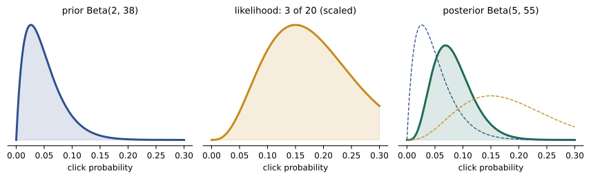
A Bayesian model has two parts: a likelihood describing how data arise given parameters, and a prior over the parameters. Consider estimating the probability \(\theta\) that a user clicks an advertisement. If \(n\) users see it and \(k\) click, the likelihood is binomial: \(p(k \mid \theta) \propto \theta^k(1 - \theta)^{n-k}\). A natural prior is the beta distribution, \(\mathrm{Beta}(\theta \mid a, b) \propto \theta^{a-1}(1 - \theta)^{b-1}\), whose mean is \(a/(a + b)\). Multiplying gives
The posterior is again a beta distribution: the data simply add the number of successes to \(a\) and failures to \(b\). The prior parameters act like pseudo-counts, so \(\mathrm{Beta}(1, 1)\), the uniform distribution, is worth two observations, and \(\mathrm{Beta}(20, 380)\) encodes a belief that the click rate is around 5%, held with the strength of 400 observations.
from scipy import stats

a, b = 2, 38                         # prior: mean 0.05, worth 40 pseudo-observations
for n, k in [(0, 0), (20, 3), (200, 18), (2000, 170)]:
    post = stats.beta(a + k, b + n - k)
    lo, hi = post.ppf([0.025, 0.975])
    mle = f"{k / n:.3f}" if n else "  -  "
    print(f"n={n:5d} k={k:4d}  MLE={mle}  posterior mean={post.mean():.3f}  "
f"95% interval=({lo:.3f}, {hi:.3f})")n= 0 k= 0 MLE= - posterior mean=0.050 95% interval=(0.006, 0.135) n= 20 k= 3 MLE=0.150 posterior mean=0.083 95% interval=(0.028, 0.165) n= 200 k= 18 MLE=0.090 posterior mean=0.083 95% interval=(0.052, 0.121) n= 2000 k= 170 MLE=0.085 posterior mean=0.084 95% interval=(0.073, 0.097)
With no data the posterior is the prior. After 20 users and 3 clicks, the maximum likelihood estimate (MLE) of 0.15 is pulled strongly toward the prior mean, and the interval is wide. As data accumulate, the posterior concentrates around the observed rate and the prior matters less and less: with 2000 observations the prior's 40 pseudo-counts are nearly irrelevant.
Conjugate priors
A prior is conjugate to a likelihood when the posterior belongs to the same family as the prior, as with the beta and binomial. Conjugacy gives closed-form updates, which is why these pairs appear constantly in practice and as building blocks of larger models:
| Likelihood | Parameter | Conjugate prior | Posterior update |
|---|---|---|---|
| Bernoulli / binomial | probability \(\theta\) | \(\mathrm{Beta}(a, b)\) | \(a + k,\; b + n - k\) |
| Categorical / multinomial | probabilities \(\boldsymbol\pi\) | \(\mathrm{Dirichlet}(\boldsymbol\alpha)\) | \(\alpha_j + n_j\) |
| Poisson | rate \(\lambda\) | \(\mathrm{Gamma}(a, b)\) | \(a + \sum x_i,\; b + n\) |
| Normal, known variance \(\sigma^2\) | mean \(\mu\) | \(\mathcal N(\mu_0, \tau_0^2)\) | precisions add; mean is precision-weighted |
| Normal, known mean | precision \(\lambda\) | \(\mathrm{Gamma}(a, b)\) | \(a + n/2,\; b + \tfrac12\sum (x_i - \mu)^2\) |
For the normal mean with known noise variance \(\sigma^2\), the posterior after \(n\) observations with sample mean \(\bar x\) is normal with
Precisions (inverse variances) add, and the posterior mean is a weighted average of the prior mean and the sample mean, each weighted by its precision. This "precision-weighted averaging" is the essence of how Bayesian updating combines information, and it reappears in Kalman filters, linear regression and Gaussian processes.
Worked problem
Combining a prior and a measurement
A sensor's offset is believed, from the manufacturer's data, to be normally distributed with mean 0 and standard deviation 2 mV. Calibration takes 4 readings with noise standard deviation 3 mV and a mean of 2.5 mV. What is the posterior distribution of the offset?
Show solution
- Prior precision: \(1/2^2 = 0.25\). Data precision: \(n/\sigma^2 = 4/9 = 0.444\).
- Posterior precision: \(0.25 + 0.444 = 0.694\), so \(\tau_n^2 = 1.44\) and \(\tau_n = 1.2\) mV.
- Posterior mean: \(1.44 \times (0 \times 0.25 + 2.5 \times 0.444) = 1.44 \times 1.111 = 1.60\) mV.
Answer: Normal with mean 1.60 mV and standard deviation 1.2 mV. The data carry a little more weight (0.444 against 0.25) than the prior, so the estimate moves 64% of the way from 0 toward 2.5.
From posterior to answers
Point estimates
A full posterior is the complete answer, but decisions often need a single number. The posterior mean minimizes expected squared error, the posterior median minimizes expected absolute error, and the posterior mode is the maximum a posteriori (MAP) estimate:
MAP estimation is maximum likelihood plus a penalty from the prior, which connects Bayesian reasoning to regularization. A zero-mean Gaussian prior on regression weights gives \(\log p(\mathbf w) = -\|\mathbf w\|^2/(2\tau^2) + \text{const}\), so MAP is ridge regression with \(\lambda = \sigma^2/\tau^2\); a Laplace prior gives the lasso. Weight decay in neural networks is a Gaussian prior in disguise. MAP, however, discards the uncertainty and depends on the parameterization, so it is a convenience rather than the Bayesian answer.
Credible intervals
A 95% credible interval contains 95% of the posterior probability, so it supports the statement "given the model and data, \(\theta\) lies in this interval with probability 0.95". This is the interpretation people usually want, and which a frequentist confidence interval does not literally provide (a confidence interval procedure covers the true value in 95% of repeated experiments). With weak priors and plenty of data the two intervals are often numerically similar.
Posterior predictive distribution
Predictions should average over parameter uncertainty rather than plug in a single estimate:
For the beta-binomial model, the probability that the next user clicks is the posterior mean \((a + k)/(a + b + n)\). With a uniform prior this is Laplace's rule of succession, \((k + 1)/(n + 2)\), which never predicts probability exactly 0 or 1 from finite data, unlike the MLE. Posterior predictive distributions are wider than plug-in predictions, correctly reflecting that the parameters are not known exactly.
Bayesian decisions: an A/B test
Posteriors answer the questions decision makers actually ask. Suppose two versions of a web page are tested: A has 120 conversions from 2400 visitors and B has 145 from 2380. Rather than a p-value, a Bayesian analysis gives the probability that B is better, and the expected gain or loss from choosing it, by sampling from the two posteriors.
import numpy as np

rng = np.random.default_rng(0)
nA, kA = 2400, 120
nB, kB = 2380, 145
pA = rng.beta(1 + kA, 1 + nA - kA, size=200_000)
pB = rng.beta(1 + kB, 1 + nB - kB, size=200_000)

lift = pB / pA - 1
print(f"P(B better than A)      = {np.mean(pB > pA):.3f}")
print(f"median relative lift     = {np.median(lift):.1%}")
print(f"95% interval for lift    = ({np.quantile(lift, 0.025):.1%}, {np.quantile(lift, 0.975):.1%})")
print(f"expected loss choosing B = {np.mean(np.maximum(pA - pB, 0)):.5f}")
print(f"expected loss choosing A = {np.mean(np.maximum(pB - pA, 0)):.5f}")P(B better than A) = 0.950 median relative lift = 21.7% 95% interval for lift = (-3.7%, 54.0%) expected loss choosing B = 0.00014 expected loss choosing A = 0.01104
The expected loss is the conversion rate we would give up, on average, by choosing a version if it is actually the worse one. A common decision rule is to stop the test when the expected loss of the leading option falls below a threshold of caring, for example 0.0005 (0.05 percentage points); here B's expected loss of 0.00014 is already below it, even though the interval for the lift still includes zero. Bayesian analyses still require care: peeking repeatedly at the results and stopping when they look good does not invalidate the posterior itself, but it does change the long-run error rates, and the prior and model assumptions must be stated.
Model comparison and the marginal likelihood
The evidence \(p(D) = \int p(D \mid \theta)\,p(\theta)\,d\theta\), ignored when computing a posterior, becomes central when comparing models. For two models \(M_1\) and \(M_2\), Bayes' theorem at the model level gives
The ratio of marginal likelihoods is the Bayes factor. The marginal likelihood is the probability the model assigned to the observed data before seeing them, averaged over its prior. A flexible model with many parameters spreads its probability over many possible data sets, so it assigns less to any particular one; it wins only if the data really need the flexibility. This automatic Occam's razor penalizes complexity without a separate penalty term. Its drawback is sensitivity to the prior: a vague prior spreads probability thinly and is penalized heavily, even when the posterior hardly depends on it.
import numpy as np
from scipy.special import betaln

# 100 coin flips with 61 heads. M1: fair coin. M2: unknown bias with a uniform prior.
n, k = 100, 61
log_ev_fair = n * np.log(0.5)
log_ev_free = betaln(1 + k, 1 + n - k) - betaln(1, 1)      # integral of theta^k (1-theta)^(n-k)
bf = np.exp(log_ev_free - log_ev_fair)
print(f"log evidence, fair coin   = {log_ev_fair:.3f}")
print(f"log evidence, free bias   = {log_ev_free:.3f}")
print(f"Bayes factor (free : fair) = {bf:.2f}")

# For comparison: the classical two-sided binomial test
from scipy.stats import binomtest
print(f"two-sided p-value = {binomtest(k, n, 0.5).pvalue:.4f}")log evidence, fair coin = -69.315 log evidence, free bias = -68.984 Bayes factor (free : fair) = 1.39 two-sided p-value = 0.0352
With 61 heads in 100 flips, the classical test rejects a fair coin at the 5% level, but the Bayes factor is only about 1.4, barely favouring the biased coin. The two approaches answer different questions: the p-value measures how surprising the data are under the fair model alone, while the Bayes factor compares how well the two specific models predicted the data. A uniform prior on the bias wastes probability on values like 0.05 or 0.95, which the data clearly rule out. Computing the marginal likelihood is usually hard, since it is an integral over all parameters; Lessons 7 and 9 present methods that approximate it.
Hierarchical models and shrinkage
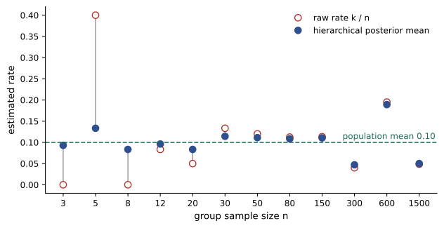
Real problems often involve many related parameters: conversion rates for hundreds of products, test scores for many schools, failure rates for many machines of the same type. Estimating each separately (no pooling) is noisy for groups with little data; assuming they are all equal (complete pooling) ignores real differences. A hierarchical model treats the group parameters as drawn from a common population distribution whose parameters are also learned:
The posterior for each \(\theta_j\) is pulled toward the population mean, strongly for small groups and weakly for large ones. This partial pooling, or shrinkage, reduces total estimation error and is one of the most practically valuable ideas in statistics: it explains why a product with 2 sales from 3 visitors should not be ranked above one with 900 from 10,000.
Worked problem
Empirical Bayes shrinkage
A population of products has conversion rates well described by \(\mathrm{Beta}(4, 36)\) (mean 0.10). Product X had 2 conversions from 3 visitors, and product Y had 900 from 10,000. Compare the raw and shrunk estimates.
Show solution
- X raw: \(2/3 = 0.667\). Shrunk: \((4 + 2)/(40 + 3) = 6/43 = 0.140\).
- Y raw: \(900/10{,}000 = 0.090\). Shrunk: \((4 + 900)/(40 + 10{,}000) = 904/10{,}040 = 0.090\).
Answer: X drops from 0.667 to 0.140, close to the population mean, because 3 visitors are worth far less than the prior's 40 pseudo-observations; Y is unchanged. Estimating \(a\) and \(b\) from all the products, then using them as the prior, is called empirical Bayes; a fully Bayesian hierarchical model places a prior on \(a\) and \(b\) as well.
How this course is organized
The twelve lessons build from foundations to applications:
- Lesson 1 (this lesson): Bayesian reasoning, conjugate models, decisions and model comparison.
- Lesson 2: standard distributions, maximum likelihood and MAP estimation, the exponential family, the multivariate Gaussian and KL divergence.
- Lesson 3: graphical models, conditional independence, exact inference and hidden Markov models.
- Lesson 4: learning graphical models, loopy belief propagation, conditional random fields and causal inference.
- Lesson 5: latent variable models and the EM algorithm.
- Lesson 6: Gaussian processes for regression and classification.
- Lesson 7: Monte Carlo sampling, MCMC and its diagnostics.
- Lesson 8: Bayesian linear regression, generalized linear models and hierarchical regression.
- Lesson 9: variational inference and variational autoencoders.
- Lesson 10: probabilistic programming, the Bayesian workflow, predictive checks and model comparison.
- Lesson 11: state-space models, Kalman filters and particle filters.
- Lesson 12: uncertainty in machine learning, calibration, conformal prediction, Bayesian optimization and a capstone project.
Common mistakes
MistakeIgnoring base rates when interpreting a positive test or classifier alert.
InsteadCombine the likelihood ratio with the prior: rare events produce mostly false positives.
MistakeReporting the MAP estimate as if it captured the Bayesian answer.
InsteadReport the posterior (or intervals and predictive distributions); MAP discards uncertainty.
MistakePlugging a point estimate into predictions.
InsteadAverage over the posterior; predictive distributions should be wider than plug-in ones.
MistakeUsing very vague priors in Bayes factor comparisons.
InsteadMarginal likelihoods are sensitive to prior width; use reasonable priors and check sensitivity.
MistakeEstimating many small groups separately.
InsteadUse hierarchical models so that small groups borrow strength from the population.
Summary and key terms
- Bayes' theorem: posterior \(\propto\) likelihood \(\times\) prior; the evidence normalizes.
- Base rates matter: rare conditions produce mostly false positives.
- Conjugate priors give closed-form updates; beta-binomial priors act as pseudo-counts.
- Normal updates add precisions and average means by precision.
- MAP equals regularized maximum likelihood (Gaussian prior = ridge, Laplace = lasso).
- Credible intervals state where the parameter lies with a given probability, given the model.
- Posterior predictive distributions average over parameter uncertainty.
- Posterior sampling gives direct answers to decision questions such as P(B better than A) and expected loss.
- Marginal likelihoods and Bayes factors compare models with an automatic Occam penalty, but depend on priors.
- Hierarchical models partially pool related groups, shrinking noisy estimates toward the population.
- Prior
- The distribution expressing beliefs about a parameter before seeing data.
- Likelihood
- The probability of the data as a function of the parameters.
- Posterior
- The distribution of the parameters given the data.
- Evidence (marginal likelihood)
- The probability of the data averaged over the prior.
- Conjugate prior
- A prior that yields a posterior in the same family.
- Pseudo-counts
- Interpretation of beta or Dirichlet prior parameters as imaginary prior observations.
- MAP estimate
- The posterior mode.
- Credible interval
- An interval containing a stated posterior probability.
- Posterior predictive
- The distribution of new data averaged over the posterior.
- Bayes factor
- The ratio of marginal likelihoods of two models.
- Hierarchical model
- A model in which group parameters share a learned population distribution.
- Shrinkage
- Pulling noisy group estimates toward a common mean.
- Empirical Bayes
- Estimating prior parameters from the data and then treating them as fixed.
Practice problems
Work each problem on paper first, then reveal the answer to check.
A fraud model flags 3% of legitimate transactions and 90% of fraudulent ones. Fraud is 0.2% of transactions. What fraction of flagged transactions are fraud?
Show answer
0.9 × 0.002 = 0.0018; 0.03 × 0.998 = 0.02994; 0.0018/(0.0018 + 0.02994) = 5.7%.
A Beta(3, 7) prior is updated with 12 successes in 20 trials. What is the posterior and its mean?
Show answer
Beta(15, 15), mean 0.5.
What is the predictive probability of success on the next trial in the previous question?
Show answer
15/30 = 0.5 (the posterior mean).
A Gamma(2, 1) prior on a Poisson rate is updated with counts 3, 5, 4. What is the posterior?
Show answer
Gamma(2 + 12, 1 + 3) = Gamma(14, 4), mean 3.5.
Prior N(10, 4²); 9 observations with σ = 6 and mean 14. Find the posterior mean and SD.
Show answer
Prior precision 1/16 = 0.0625; data 9/36 = 0.25; total 0.3125 → var 3.2, SD 1.79; mean 3.2 × (10 × 0.0625 + 14 × 0.25) = 13.2.
Show that MAP with a Gaussian prior N(0, τ²I) on linear regression weights and noise variance σ² is ridge regression.
Show answer
Maximize −‖y − Xw‖²/(2σ²) − ‖w‖²/(2τ²); multiply by −2σ²: minimize ‖y − Xw‖² + (σ²/τ²)‖w‖², ridge with λ = σ²/τ².
With a uniform prior, 0 failures were seen in 30 trials. What does Laplace's rule give for the failure probability?
Show answer
(0 + 1)/(30 + 2) = 0.031.
Why does a model with more parameters not automatically have a higher marginal likelihood?
Show answer
It spreads its prior predictive probability over more possible data sets, so it assigns less probability to the observed data unless its flexibility is needed.
Population prior Beta(10, 90). Group A: 5/10; group B: 500/1000. Shrunk estimates?
Show answer
A: 15/110 = 0.136; B: 510/1100 = 0.464.
What is the difference between a 95% credible interval and a 95% confidence interval?
Show answer
The credible interval contains the parameter with posterior probability 0.95 given the data and model; the confidence interval procedure covers the true value in 95% of repeated experiments.
Lesson quiz · 5 questions
Score 60% or more to complete this lesson.
Create a free account to save your progress, take quizzes and earn a certificate.