State-space models and filtering

Many problems involve a quantity that changes over time and can only be observed indirectly and noisily: the position of a vehicle from GPS fixes, the charge of a battery from its voltage, the number of infected people from reported cases, the health of a machine from vibration readings. State-space models describe such systems with a hidden state that evolves according to dynamics and observations that depend on the current state. Hidden Markov models (Lesson 3) are the version with a discrete state. This lesson treats continuous states: the Kalman filter for linear Gaussian systems, smoothing and parameter learning, extensions to nonlinear systems, and particle filters, the sequential Monte Carlo methods introduced in Lesson 7 applied to tracking. It ends with the link to modern sequence models in deep learning.

The state-space model

A state-space model has two equations. The state \(\mathbf{x}_t\) evolves by a transition model, and each observation \(\mathbf{y}_t\) depends on the current state through an observation model:

This is the linear Gaussian state-space model, also called a linear dynamical system. Its graph is the same chain as an HMM: each state depends only on the previous one, and each observation only on its state. A tracking example: the state is position and velocity, \(\mathbf{x} = (p, v)\); the transition moves position by velocity times the time step and lets velocity drift randomly (a constant-velocity model); and the observation measures position with noise.

Three inference tasks recur, matching those for HMMs:

• Filtering: \(p(\mathbf{x}_t \mid \mathbf{y}_{1:t})\), the current state given observations so far, for real-time estimation and control.
• Smoothing: \(p(\mathbf{x}_t \mid \mathbf{y}_{1:T})\), using later observations as well, for offline analysis.
• Prediction: \(p(\mathbf{x}_{t+k} \mid \mathbf{y}_{1:t})\), for forecasting.

The Kalman filter

In a linear Gaussian model, every filtering distribution is Gaussian, \(p(\mathbf{x}_t \mid \mathbf{y}_{1:t}) = \mathcal{N}(\mathbf{m}_t, \mathbf{P}_t)\), so the filter only needs to track a mean and a covariance. Each time step has two stages. Prediction pushes the previous estimate through the dynamics, adding process noise:

The update conditions on the new observation, using the Gaussian conditioning rule of Lesson 2. The difference between the observation and its prediction is the innovation \(\mathbf{e}_t = \mathbf{y}_t - \mathbf{H}\mathbf{m}_{t|t-1}\), with covariance \(\mathbf{S}_t = \mathbf{H}\mathbf{P}_{t|t-1}\mathbf{H}^\top + \mathbf{R}\). The Kalman gain decides how much of the innovation to believe:

When measurements are noisy compared with the predicted uncertainty, the gain is small and the filter trusts its prediction; when the prediction is uncertain, the gain is large and the filter follows the measurements. The covariance recursion does not involve the observations, so the gains can be precomputed, and for a time-invariant system they converge to a steady-state value.

import numpy as np

rng = np.random.default_rng(12)
dt, T = 1.0, 50
F = np.array([[1, dt], [0, 1]])                       # state: position and velocity
H = np.array([[1.0, 0.0]])                            # we measure position only
q, r = 0.05, 4.0                                      # process and measurement noise variances
Q = q * np.array([[dt ** 3 / 3, dt ** 2 / 2], [dt ** 2 / 2, dt]])
R = np.array([[r]])

x = np.array([0.0, 1.0]); truth, obs = [], []
for t in range(T):
    x = F @ x + rng.multivariate_normal([0, 0], Q)
    truth.append(x.copy()); obs.append(H @ x + rng.normal(0, np.sqrt(r), 1))
truth, obs = np.array(truth), np.array(obs).ravel()

m, P = np.array([0.0, 0.0]), np.diag([10.0, 10.0])
est = []
for z in obs:
    m, P = F @ m, F @ P @ F.T + Q                     # predict
    S = H @ P @ H.T + R                               # innovation variance
    K = P @ H.T / S                                   # Kalman gain
    m = m + (K * (z - H @ m)).ravel()                 # update with the measurement
    P = (np.eye(2) - K @ H) @ P
    est.append(m.copy())
est = np.array(est)
rmse = lambda a: np.sqrt(np.mean((a - truth[:, 0]) ** 2))
print(f"position RMSE: raw measurements {rmse(obs):.2f}, Kalman filter {rmse(est[:, 0]):.2f}")
print(f"final velocity estimate {est[-1, 1]:.2f} +/- {1.96 * np.sqrt(P[1, 1]):.2f} (true {truth[-1, 1]:.2f})")
print(f"steady-state gain for position: {K[0, 0]:.2f}")

position RMSE: raw measurements 1.75, Kalman filter 1.09
final velocity estimate -0.91 +/- 0.85 (true -0.85)
steady-state gain for position: 0.38

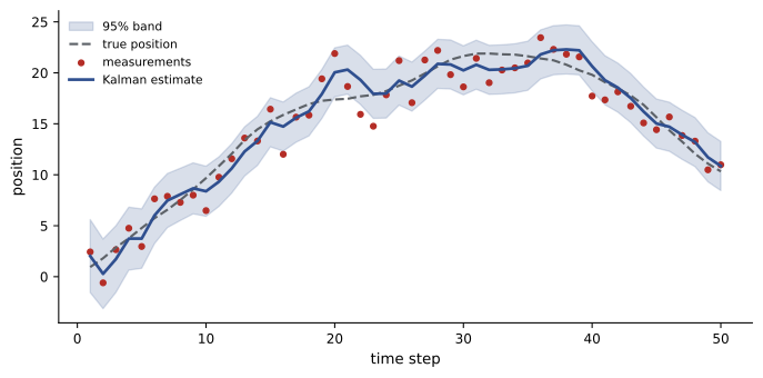
The filter cuts the position error by more than a third compared with the raw measurements, and it estimates velocity, which is never measured, by combining successive positions with the dynamics model. This ability to infer unmeasured states is why Kalman filters run in every GPS receiver, aircraft navigation system, phone motion sensor and battery management system.

Smoothing and learning parameters

For offline analysis, the Rauch-Tung-Striebel (RTS) smoother adds a backward pass after filtering. Starting from the final filtered estimate, it revises each earlier estimate using the information from later observations, producing \(p(\mathbf{x}_t \mid \mathbf{y}_{1:T})\), with lower variance than the filtered estimate, especially in the middle of the series. It is the continuous analogue of the forward-backward algorithm for HMMs.

The model matrices, especially the noise covariances \(\mathbf{Q}\) and \(\mathbf{R}\), are rarely known exactly, and the filter's performance depends strongly on them. Too small a \(\mathbf{Q}\) makes the filter sluggish and overconfident, ignoring real changes; too large a \(\mathbf{Q}\) makes it jittery. Two standard ways of learning them:

• Maximum likelihood using the innovations: the log-likelihood of the data is \(\sum_t \log\mathcal{N}(\mathbf{e}_t; \mathbf{0}, \mathbf{S}_t)\), computed by one run of the filter, and can be maximized numerically.
• EM (Lesson 5): the E-step runs the smoother to get expected states and their covariances, and the M-step re-estimates \(\mathbf{F}\), \(\mathbf{H}\), \(\mathbf{Q}\) and \(\mathbf{R}\) in closed form.

A useful check on a tuned filter: the normalized innovations \(\mathbf{e}_t^\top\mathbf{S}_t^{-1}\mathbf{e}_t\) should average about the dimension of \(\mathbf{y}\) and show no autocorrelation. Innovations that are consistently too large signal that the filter is overconfident; autocorrelated innovations signal missing dynamics.

Nonlinear systems

Many systems are nonlinear: a radar measures range and bearing, nonlinear functions of position; a battery's voltage depends nonlinearly on its charge; epidemic dynamics are multiplicative. With nonlinear transition \(f\) or observation \(h\), Gaussians no longer stay Gaussian, and approximations are needed.

• The extended Kalman filter (EKF) linearizes \(f\) and \(h\) around the current estimate using their Jacobians and applies the Kalman equations to the linearized system. It is cheap and widely used, but can diverge when the nonlinearity is strong relative to the uncertainty.
• The unscented Kalman filter (UKF) passes a small set of deterministically chosen sigma points (\(2n + 1\) for an \(n\)-dimensional state) through the exact nonlinear functions and fits a Gaussian to the results. It needs no Jacobians and captures the mean and covariance more accurately, at similar cost.

Both still represent the belief by a single Gaussian, so they fail when the true posterior is multimodal, for example when a measurement cannot distinguish two positions.

Particle filters

Particle filters represent the filtering distribution by a set of weighted samples (particles), so they can follow any shape of distribution, including several modes. The bootstrap particle filter repeats three steps at each time:

• Propagate: move each particle through the transition model, including random process noise.
• Weight: set each particle's weight proportional to the likelihood of the new observation given that particle, \(w^{(i)} \propto p(\mathbf{y}_t \mid \mathbf{x}_t^{(i)})\), and normalize.
• Resample: draw a new set of particles with probabilities equal to the weights, so that particles in likely regions multiply and unlikely ones die out.

Estimates are weighted averages over the particles. Without resampling, almost all the weight would soon concentrate on a single particle (weight degeneracy). Resampling fixes that but reduces diversity, so it is often done only when the effective sample size \(1/\sum_i (w^{(i)})^2\) falls below a threshold such as half the number of particles.

import numpy as np

rng = np.random.default_rng(13)
# Nonlinear benchmark model: x_t = 0.5 x + 25 x / (1 + x^2) + 8 cos(1.2 t) + noise; y_t = x^2 / 20 + noise
T, N = 60, 2000
def step(x, t):
    return 0.5 * x + 25 * x / (1 + x ** 2) + 8 * np.cos(1.2 * t)
x, xs, ys = 0.1, [], []
for t in range(1, T + 1):
    x = step(x, t) + rng.normal(0, np.sqrt(10))
    xs.append(x); ys.append(x ** 2 / 20 + rng.normal(0, 1))
xs, ys = np.array(xs), np.array(ys)

particles = rng.normal(0, 2, N)
means, ess_low = [], 0
for t in range(1, T + 1):
    particles = step(particles, t) + rng.normal(0, np.sqrt(10), N)       # propagate
    logw = -0.5 * (ys[t - 1] - particles ** 2 / 20) ** 2                 # weight by the likelihood
    w = np.exp(logw - logw.max()); w /= w.sum()
    means.append(np.sum(w * particles))
    if 1 / np.sum(w ** 2) < N / 2: ess_low += 1
    particles = particles[rng.choice(N, N, p=w)]                         # resample
means = np.array(means)
print(f"RMSE of particle filter mean: {np.sqrt(np.mean((means - xs) ** 2)):.2f} (state sd {xs.std():.2f})")
print(f"steps where effective sample size fell below N/2: {ess_low} of {T}")
sign_ok = np.mean(np.sign(means) == np.sign(xs))
print(f"sign of the state recovered at {sign_ok:.0%} of steps (y depends on x squared, so the sign is ambiguous)")

RMSE of particle filter mean: 3.33 (state sd 10.85)
steps where effective sample size fell below N/2: 44 of 60
sign of the state recovered at 87% of steps (y depends on x squared, so the sign is ambiguous)

Because the observation depends on \(x^2\), a single measurement cannot tell \(+x\) from \(-x\); the posterior is often bimodal, and any Gaussian filter would fail. The particle filter keeps both modes alive until the dynamics resolve the ambiguity, recovering the sign most of the time and tracking the state with an error well below its natural spread. The effective sample size often fell below half, showing why adaptive resampling is necessary.

Particle filters need many particles when the state has many dimensions, because the volume to cover grows exponentially; practical variants use better proposals (incorporating the current observation), Rao-Blackwellization (handling linear parts of the state exactly with Kalman filters) and particle MCMC for learning parameters. Their applications include robot localization (the Monte Carlo localization used by mobile robots), target tracking in clutter, and epidemic and financial models with non-Gaussian dynamics.

State-space models in modern machine learning

The state-space idea has returned in deep learning. Recurrent neural networks carry a hidden state forward in time, like a filter with learned nonlinear dynamics but without explicit uncertainty. Deep state-space models (structured state-space sequence models such as S4, and selective models such as Mamba) build sequence layers from linear state-space recurrences \(\mathbf{x}_t = \bar{\mathbf{A}}\mathbf{x}_{t-1} + \bar{\mathbf{B}}u_t\), \(y_t = \mathbf{C}\mathbf{x}_t\), whose linearity allows the whole sequence to be computed in parallel during training and handles very long contexts efficiently. Probabilistic deep state-space models combine neural transition and observation functions with variational inference (Lesson 9), learning dynamics from data while retaining uncertainty. And the Kalman filter remains the standard baseline for any forecasting or tracking problem with roughly linear dynamics, often hard to beat when data are limited.