Latent variables and EM

Many patterns in data are best explained by quantities we never observe. Customers belong to segments that no database records; a document is about topics that are not labelled; an image of a digit was written in one of several styles; a machine is in a health state that can only be inferred from its vibration. Latent variable models make these hidden quantities explicit as random variables, which turns vague notions such as "clusters" or "topics" into precise probabilistic models that can be fitted, compared and used for prediction. The difficulty is that the likelihood of the observed data involves a sum or integral over the latent variables, which is awkward to maximize directly. The expectation-maximization (EM) algorithm solves this elegantly. This lesson develops mixture models, the EM algorithm and why it works, practical issues such as initialization and choosing the number of components, and extensions to missing data and other latent variable models.

Mixture models

A mixture model assumes that each data point was generated by first choosing one of \(K\) components at random, then drawing from that component's distribution. Introducing a latent variable \(z_n \in \{1, \ldots, K\}\) for each point \(x_n\):

This is a Gaussian mixture model (GMM). Summing out the latent variable gives the marginal density of an observation, a weighted sum of Gaussians:

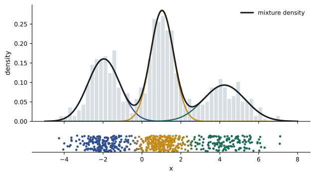
Mixtures are flexible density estimators: with enough components a GMM can approximate any smooth density. They also provide soft clustering, because Bayes' theorem gives the posterior probability that point \(n\) came from component \(k\), called its responsibility:

Unlike k-means, which assigns each point wholly to one cluster, a GMM expresses uncertainty about points between clusters, allows clusters of different sizes and shapes through the covariances, and gives a likelihood that can be used to compare models.

Why direct maximization is hard

The log-likelihood of the data is

The logarithm of a sum does not simplify, so setting derivatives to zero gives coupled equations without a closed-form solution. If the latent assignments \(z_n\) were known, the problem would be easy: the log-likelihood would split into separate terms for each component, and each \(\mu_k\) would be the mean of its points, each \(\Sigma_k\) their covariance and each \(\pi_k\) the fraction of points assigned. EM exploits this by alternating between guessing the assignments (softly) and solving the easy problem.

Maximum likelihood for GMMs also has a pathology: if one component's mean sits exactly on a data point and its variance shrinks toward zero, the likelihood goes to infinity. Practical implementations add a small value to the diagonal of each covariance (a regularizer that can be seen as a weak prior), or use a Bayesian treatment.

The EM algorithm

EM alternates two steps until the log-likelihood stops improving:

• E-step: with the current parameters, compute the responsibilities \(r_{nk}\) for every point and component.
• M-step: re-estimate the parameters as if the responsibilities were fractional counts of assignments.

For a GMM, with \(N_k = \sum_n r_{nk}\) the effective number of points in component \(k\), the M-step is

These are exactly the weighted versions of the formulas for known assignments.

import numpy as np
from scipy.stats import norm

rng = np.random.default_rng(3)
x = np.concatenate([rng.normal(-2, 0.8, 200), rng.normal(1, 0.6, 250), rng.normal(4, 1.2, 150)])

K = 3
pi = np.full(K, 1 / K); mu = np.array([-1.0, 0.0, 1.0]); sd = np.ones(K)
for it in range(1, 61):
    dens = pi * norm.pdf(x[:, None], mu, sd)          # N x K
    ll = np.log(dens.sum(axis=1)).sum()
    r = dens / dens.sum(axis=1, keepdims=True)         # E-step: responsibilities
    Nk = r.sum(axis=0)                                 # M-step
    pi = Nk / len(x)
    mu = (r * x[:, None]).sum(axis=0) / Nk
    sd = np.sqrt((r * (x[:, None] - mu) ** 2).sum(axis=0) / Nk + 1e-6)
    if it in (1, 2, 5, 10, 20, 40, 60):
        print(f"iter {it:2d}  loglik {ll:9.3f}  mu {np.round(mu, 2)}  sd {np.round(sd, 2)}  pi {np.round(pi, 2)}")

iter  1  loglik -2043.914  mu [-1.74  0.23  2.63]  sd [1.2  1.43 1.83]  pi [0.3  0.22 0.49]
iter  2  loglik -1375.300  mu [-1.8   0.35  2.59]  sd [1.12 1.36 1.9 ]  pi [0.29 0.23 0.48]
iter  5  loglik -1350.276  mu [-2.08  0.71  2.6 ]  sd [0.79 0.98 1.98]  pi [0.28 0.25 0.47]
iter 10  loglik -1303.856  mu [-2.04  0.95  2.99]  sd [0.76 0.52 1.95]  pi [0.31 0.31 0.39]
iter 20  loglik -1293.553  mu [-1.95  0.97  3.71]  sd [0.83 0.52 1.49]  pi [0.34 0.36 0.3 ]
iter 40  loglik -1285.837  mu [-1.96  1.03  4.23]  sd [0.82 0.59 1.07]  pi [0.33 0.42 0.24]
iter 60  loglik -1285.835  mu [-1.96  1.03  4.23]  sd [0.82 0.59 1.07]  pi [0.33 0.42 0.24]

The log-likelihood rises at every iteration, quickly at first and then slowly, and the parameters converge close to those used to generate the data (means −2, 1 and 4; standard deviations 0.8, 0.6 and 1.2; weights 0.33, 0.42 and 0.25). The monotone increase is not a coincidence, and it is the best test of an EM implementation: if the log-likelihood ever decreases, there is a bug.

Why EM works

For any distribution \(q(z)\) over the latent variables, Jensen's inequality gives a lower bound on the log-likelihood of one data point:

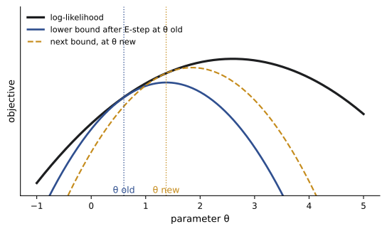
The gap between the two sides is exactly the Kullback-Leibler divergence \(\mathrm{KL}(q(z)\,\|\,p(z \mid x, \theta))\), which is non-negative and zero only when \(q\) equals the posterior. So \(\log p(x \mid \theta) = \mathcal L(q, \theta) + \mathrm{KL}(q \,\|\, p(z \mid x, \theta))\). EM is coordinate ascent on the lower bound \(\mathcal L\):

• The E-step sets \(q(z) = p(z \mid x, \theta^{\mathrm{old}})\), which makes the KL term zero, so the bound touches the log-likelihood at the current parameters.
• The M-step maximizes \(\mathcal L(q, \theta)\) over \(\theta\) with \(q\) fixed, which amounts to maximizing the expected complete-data log-likelihood \(\mathbb{E}_q[\log p(x, z \mid \theta)]\), usually easy because it has the same form as the known-assignment problem.

Since the bound equals the log-likelihood after the E-step and the M-step can only raise the bound, the log-likelihood cannot decrease. This lower bound, the evidence lower bound or ELBO, is also the starting point of variational inference in Lesson 9, where \(q\) is restricted to a tractable family because the exact posterior is unavailable.

Practical issues

Local optima and initialization

EM converges to a local maximum (or saddle point) of the likelihood, and mixture likelihoods have many: components can split a true cluster in two while another component covers two true clusters. Results depend on initialization. Standard practice is to initialize from k-means (itself initialized with k-means++), to run EM from several starting points and keep the solution with the highest log-likelihood, and to check that solutions make sense.

import numpy as np
from sklearn.mixture import GaussianMixture

rng = np.random.default_rng(7)
centres = np.array([[0, 0], [5, 0], [0, 5], [5, 5], [2.5, 9]])
X = np.vstack([c + rng.normal(scale=0.9, size=(120, 2)) for c in centres])

print("single initializations from random data points (K=5):")
for seed in range(8):
    g = GaussianMixture(5, init_params="random_from_data", n_init=1, random_state=seed, max_iter=500).fit(X)
    print(f"  seed {seed}: average loglik per point {g.score(X):.4f}, converged in {g.n_iter_} iterations")
g = GaussianMixture(5, init_params="kmeans", n_init=10, random_state=0).fit(X)
print(f"k-means init, best of 10: {g.score(X):.4f}")

single initializations from random data points (K=5):
  seed 0: average loglik per point -4.2367, converged in 12 iterations
  seed 1: average loglik per point -4.2930, converged in 25 iterations
  seed 2: average loglik per point -4.2384, converged in 11 iterations
  seed 3: average loglik per point -4.2336, converged in 11 iterations
  seed 4: average loglik per point -4.2797, converged in 7 iterations
  seed 5: average loglik per point -4.1010, converged in 16 iterations
  seed 6: average loglik per point -4.3308, converged in 16 iterations
  seed 7: average loglik per point -4.1010, converged in 12 iterations
k-means init, best of 10: -4.1010

Only two of the eight random starts reach the best solution, with an average log-likelihood of about −4.10 per point; the others stop at clearly worse local optima, in which two true clusters share one component while another true cluster is split between two. Initializing from k-means and keeping the best of several runs finds the good solution reliably.

Choosing the number of components

The likelihood always increases with more components, so it cannot choose \(K\) by itself. Common approaches are held-out likelihood (fit on training data, evaluate on validation data) and information criteria that penalize parameters. The Bayesian information criterion is

where \(p\) is the number of free parameters; lower is better. BIC approximates \(-2\) times the log marginal likelihood of Lesson 1 for large \(N\), so it inherits the Bayesian Occam penalty. For a GMM in \(d\) dimensions with full covariances, \(p = K(d + d(d+1)/2) + K - 1\).

import numpy as np
from sklearn.mixture import GaussianMixture

rng = np.random.default_rng(7)
centres = np.array([[0, 0], [5, 0], [0, 5], [5, 5], [2.5, 9]])
X = np.vstack([c + rng.normal(scale=0.9, size=(120, 2)) for c in centres])
rng.shuffle(X)
train, valid = X[:450], X[450:]

for K in range(1, 9):
    g = GaussianMixture(K, n_init=5, random_state=0).fit(train)
    p = K * (2 + 3) + K - 1
    print(f"K={K}: params {p:2d}  BIC {g.bic(train):8.1f}  train loglik/pt {g.score(train):7.3f}  "
          f"valid loglik/pt {g.score(valid):7.3f}")

K=1: params  5  BIC   4509.2  train loglik/pt  -4.976  valid loglik/pt  -4.997
K=2: params 11  BIC   4304.2  train loglik/pt  -4.708  valid loglik/pt  -4.772
K=3: params 17  BIC   4033.2  train loglik/pt  -4.366  valid loglik/pt  -4.521
K=4: params 23  BIC   3928.2  train loglik/pt  -4.208  valid loglik/pt  -4.337
K=5: params 29  BIC   3850.5  train loglik/pt  -4.082  valid loglik/pt  -4.184
K=6: params 35  BIC   3877.4  train loglik/pt  -4.071  valid loglik/pt  -4.206
K=7: params 41  BIC   3911.3  train loglik/pt  -4.068  valid loglik/pt  -4.211
K=8: params 47  BIC   3944.5  train loglik/pt  -4.064  valid loglik/pt  -4.210

Training likelihood keeps rising with \(K\), but BIC reaches its minimum at the true value of five, and validation likelihood stops improving there. In real data there is rarely a single true \(K\); different criteria may disagree, and the choice should also reflect the purpose, such as the number of customer segments a marketing team can act on.

Relationship to k-means

If all components share a covariance \(\sigma^2 I\) and \(\sigma \to 0\), the responsibilities become hard 0-or-1 assignments to the nearest mean, the E-step becomes the k-means assignment step and the M-step becomes the k-means update. K-means is thus the zero-variance limit of EM for a GMM. This explains its implicit assumptions: spherical clusters of similar size and spread.

EM beyond mixtures

EM applies whenever the complete-data likelihood is easy and the latent variables can be inferred:

• Missing data: treat missing entries as latent. For multivariate Gaussian data, the E-step fills in the conditional expectations of the missing values (and their covariance), and the M-step recomputes the mean and covariance, giving maximum likelihood estimates without discarding incomplete rows. This is far better than mean imputation, which shrinks variances and distorts correlations.
• Hidden Markov models: the Baum-Welch algorithm uses the forward-backward algorithm of Lesson 3 for the E-step, giving expected state occupancies and transition counts, and re-estimates the transition and emission probabilities in the M-step.
• Factor analysis and probabilistic PCA: continuous latent variables \(\mathbf z \sim \mathcal N(0, I)\) generate observations \(\mathbf x = W\mathbf z + \boldsymbol\mu + \boldsymbol\epsilon\). EM fits \(W\) without computing a full covariance eigendecomposition and handles missing values naturally; probabilistic PCA recovers ordinary PCA as the noise goes to zero.
• Topic models: latent Dirichlet allocation represents each document as a mixture of topics and each topic as a distribution over words; its posterior is intractable, so it is fitted with variational EM (Lesson 9) or Gibbs sampling (Lesson 7).

Variants extend EM when the steps are hard: generalized EM only improves (rather than maximizes) the bound in the M-step; stochastic and online EM update with mini-batches; and Monte Carlo EM approximates the E-step by sampling. When the E-step posterior itself is intractable, variational EM replaces it with the best approximation from a tractable family, which is the subject of Lesson 9.

The ELBO introduced here returns in Lesson 9 as the objective of variational inference, and Lesson 11 uses EM to learn the noise parameters of state-space models.