Processing data at scale

Methods that work on a laptop with a few hundred megabytes of data can fail completely at a few hundred gigabytes: the data no longer fits in memory, a single processor takes days, and a query that scans everything costs real money in a cloud warehouse. Yet most "big data" problems can be handled with a small set of ideas: use compact data types, read only what you need, process in chunks, split work across machines by key, and accept approximate answers where exact ones are too costly. This lesson explains these ideas, the systems that implement them, and how to decide when a problem actually needs them.

How big is big?

A useful first step is to estimate size. A table of \(n\) rows and \(c\) numeric columns of 8 bytes needs about \(8nc\) bytes in memory; strings stored as Python objects take far more. Libraries such as pandas typically need two to five times the data size in free memory to work comfortably, because operations create copies. A laptop with 16 GB of memory therefore handles tables up to a few gigabytes in pandas.

import numpy as np
import pandas as pd

rng = np.random.default_rng(0)
n = 1_000_000
df = pd.DataFrame({
    "user_id": rng.integers(0, 50_000, n),
    "country": rng.choice(["CA", "US", "MX", "FR", "DE"], n),
    "device": rng.choice(["mobile", "desktop", "tablet"], n, p=[0.6, 0.3, 0.1]),
    "clicks": rng.integers(0, 40, n),
    "spend": rng.gamma(2.0, 10.0, n),
})

def mb(frame):
    return frame.memory_usage(deep=True).sum() / 1e6

print(f"default types: {mb(df):6.1f} MB")
small = df.assign(
    user_id=df["user_id"].astype("int32"),
    country=df["country"].astype("category"),
    device=df["device"].astype("category"),
    clicks=df["clicks"].astype("int8"),
    spend=df["spend"].astype("float32"),
)
print(f"compact types: {mb(small):6.1f} MB")
print(small.memory_usage(deep=True).div(1e6).round(1).to_string())

default types:  130.3 MB
compact types:   11.0 MB
Index      0.0
user_id    4.0
country    1.0
device     1.0
clicks     1.0
spend      4.0

Choosing types cut memory by more than ten times. Most of the default size was the string columns, stored as Python objects; categories store each distinct value once and use small integer codes for the rows. Before reaching for a cluster, it is worth checking whether compact types and selecting only needed columns make the data fit.

Columnar storage and partitioning

Analytical data is usually stored in columnar formats such as Parquet and ORC (Lesson 8): the values of each column are stored together, compressed, with statistics (minimum, maximum, count) for each block. Three techniques make reading such data fast:

• Column pruning: a query that uses 3 of 80 columns reads only those 3.
• Predicate pushdown: block statistics let the reader skip blocks that cannot match a filter, for example blocks whose maximum date is before the requested range.
• Partitioning: files are organized into directories by a key such as date (for example, events/date=2026-10-21/), so a query on one day reads one directory.

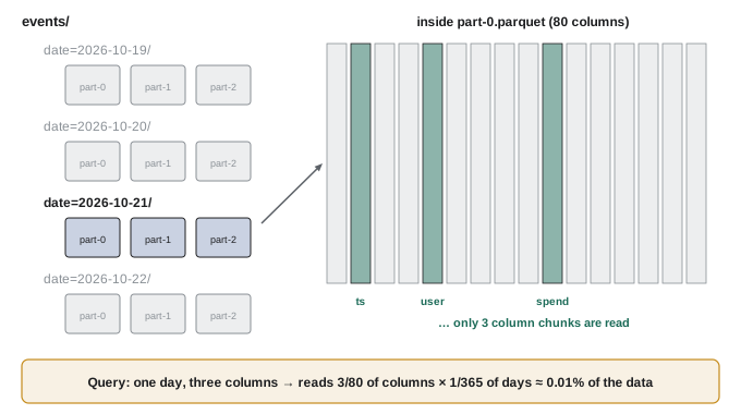
Partition keys should match common filters and give partitions of reasonable size, typically hundreds of megabytes to a few gigabytes. Partitioning by a key with millions of values creates millions of tiny files, which is slow; partitioning by a rarely filtered key does not help.

Processing in chunks

When data does not fit in memory but the computation only needs a summary, it can be streamed: read a chunk, update running totals, discard the chunk, repeat. Many statistics combine exactly across chunks: counts, sums, minimums and maximums, and therefore means and variances (keeping sums of squares, or using a numerically stable update). Others, such as exact medians and distinct counts, do not, and need either a second pass, sorting, or an approximation.

import io
import numpy as np
import pandas as pd

# Build a CSV in memory to stand in for a file too large to load at once
rng = np.random.default_rng(1)
big = pd.DataFrame({"store": rng.integers(1, 6, 200_000), "sales": rng.gamma(3.0, 20.0, 200_000)})
buf = io.StringIO()
big.to_csv(buf, index=False)
buf.seek(0)

# Stream it in chunks, keeping only running sums and counts per store
sums, counts = {}, {}
for chunk in pd.read_csv(buf, chunksize=50_000):
    g = chunk.groupby("store")["sales"].agg(["sum", "count"])
    for store, row in g.iterrows():
        sums[store] = sums.get(store, 0.0) + row["sum"]
        counts[store] = counts.get(store, 0) + int(row["count"])

streamed = pd.Series({s: sums[s] / counts[s] for s in sorted(sums)}).round(3)
direct = big.groupby("store")["sales"].mean().round(3)
print(pd.DataFrame({"streamed_mean": streamed, "in_memory_mean": direct}))
print("identical:", bool((streamed == direct).all()))

   streamed_mean  in_memory_mean
1         59.782          59.782
2         60.135          60.135
3         59.676          59.676
4         59.994          59.994
5         59.826          59.826
identical: True

The key design point is to carry mergeable state (sums and counts) rather than results (means): the mean of chunk means is wrong when chunks have different sizes, but the sum of sums divided by the sum of counts is always right.

Distributed processing

When one machine is too slow, the work is spread over many. Distributed engines such as Apache Spark, Dask, Ray and the query engines inside cloud warehouses all rest on the split-apply-combine pattern popularized by MapReduce:

• Map: each worker processes its share of the input independently, producing key-value pairs (and usually combining them locally first).
• Shuffle: pairs are sent over the network so that all pairs with the same key reach the same worker, chosen by hashing the key.
• Reduce: each worker combines the values for its keys.

import zlib
from collections import Counter, defaultdict

import numpy as np

rng = np.random.default_rng(2)
# Page-view events; one very popular page creates skew
pages = np.where(rng.random(100_000) < 0.4, "home", rng.choice([f"p{i}" for i in range(500)], 100_000))

workers = 4
def partition(key):
    return zlib.crc32(key.encode()) % workers     # stable hash, same on every machine

# Map: each input split counts locally (a combiner), then sends counts by key to a reducer
splits = np.array_split(pages, 8)
shuffled = defaultdict(Counter)
for split in splits:
    local = Counter(split.tolist())
    for key, c in local.items():
        shuffled[partition(key)][key] += c

# Reduce: each worker owns some keys and sums their counts
totals = Counter()
for w in range(workers):
    totals.update(shuffled[w])
print("top pages:", totals.most_common(3))

# Skew: events handled per reducer
load = [sum(shuffled[w].values()) for w in range(workers)]
print("events per reducer:", load, " max/mean =", round(max(load) / (sum(load) / workers), 2))

top pages: [('home', 39951), ('p137', 148), ('p307', 148)]
events per reducer: [54923, 15082, 15006, 14989]  max/mean = 2.2

The shuffle is usually the most expensive step, because it moves data across the network, and skew is the most common performance problem. In the example, 40% of events have the key "home", so the reducer that owns it does nearly four times the work of the others, and the whole job waits for it. Remedies include combining locally before the shuffle (as the example does), splitting hot keys into several sub-keys ("salting") and recombining, or handling known hot keys separately.

Joins in distributed systems follow the same pattern. A broadcast join sends a small table to every worker so the large table never moves; a shuffle join redistributes both tables by key. Knowing which one the engine chooses, from its query plan, explains most slow joins.

Approximate algorithms

Some questions are expensive to answer exactly at scale but cheap to answer approximately with small, mergeable summaries called sketches:

• Distinct counts: HyperLogLog and related sketches estimate the number of distinct values to within about 1% to 2% using a few kilobytes, whatever the data size.
• Quantiles: t-digest and KLL sketches estimate medians and percentiles with bounded error.
• Frequencies: Count-Min sketches estimate how often each item appears and find heavy hitters.
• Sampling: reservoir sampling keeps a uniform random sample of fixed size from a stream of unknown length.

import hashlib
import random

import numpy as np

random.seed(5)
stream = (f"user{random.randint(1, 300_000)}" for _ in range(1_000_000))

# Reservoir sampling: a uniform sample of fixed size from a stream of unknown length
k, reservoir = 5, []
# Distinct count by k minimum values (KMV): keep the smallest hash values seen
m, mins = 256, set()
seen = set()           # exact answer, only possible here because the demo is small

for i, item in enumerate(stream):
    if i < k:
        reservoir.append(item)
    else:
        j = random.randint(0, i)
        if j < k:
            reservoir[j] = item
    h = int(hashlib.blake2b(item.encode(), digest_size=8).hexdigest(), 16) / 2 ** 64
    if len(mins) < m:
        mins.add(h)
    elif h < max(mins) and h not in mins:
        mins.remove(max(mins))
        mins.add(h)
    seen.add(item)

estimate = (m - 1) / max(mins)
print("reservoir sample:", reservoir)
print(f"exact distinct users {len(seen):,}; KMV estimate {estimate:,.0f}; error {100 * (estimate / len(seen) - 1):+.1f}%")
print(f"memory: exact set holds {len(seen):,} items; sketch holds {m}")

reservoir sample: ['user149127', 'user243468', 'user276187', 'user188861', 'user66191']
exact distinct users 289,345; KMV estimate 286,545; error -1.0%
memory: exact set holds 289,345 items; sketch holds 256

The sketch works because hashes are spread uniformly between 0 and 1: if \(n\) distinct values are hashed, the \(k\)-th smallest hash is about \(k/n\), so \(n \approx (k-1)/h_{(k)}\). Sketches from different partitions can be merged by keeping the smallest values of their union, which is why warehouses offer approximate distinct counts as a fast built-in function.

Choosing tools

More infrastructure is not always better. A practical progression is:

• Small (up to a few GB): pandas or similar on one machine, with compact types.
• Medium (tens to hundreds of GB): a columnar, multi-threaded engine on one machine (for example DuckDB or Polars), or a cloud warehouse, reading Parquet with pruning and pushdown.
• Large (terabytes and up, or heavy computation): a distributed engine (Spark, Dask, Ray) or the warehouse's own distributed execution.

A single modern server with hundreds of gigabytes of memory and dozens of cores handles workloads that once needed clusters, with less complexity. Distributed systems add overhead for scheduling, shuffles and failures, and are worth it when the data or computation genuinely exceeds one machine, or when the organization already runs them.

Sampling is the other underused tool. Exploration, feature design and model selection can usually be done on a well-designed sample (stratified where needed, Lesson 1), with only the final pipeline run on all the data.