Data sources and collection

A machine learning model is a summary of the data it was trained on. If the data is biased, stale, mislabelled or collected in a way that leaks the answer, no model architecture will fix it. Practitioners routinely report that most of the work in an applied machine learning project goes into finding, collecting, cleaning and understanding data rather than into modelling, and many of the most consequential failures of deployed systems trace back to data decisions made early and never revisited.

This course covers that work. This lesson is about where data comes from and how to collect it responsibly and representatively. The section at the end of this lesson shows how the remaining eleven lessons build on it. The code uses Python with pandas, NumPy, scikit-learn and Matplotlib, as introduced in AI-110, and SQL as introduced in CMPUT-291.

Kinds of data

Data comes in three broad forms, each needing different tools:

• Structured data fits in tables with fixed columns and types: transactions, sensor readings, customer records. It lives in relational databases and spreadsheets and is queried with SQL or pandas.
• Semi-structured data has structure that varies from record to record: JSON documents from web APIs, log lines, XML, event streams. It must be parsed and often flattened before analysis.
• Unstructured data has no predefined fields: free text, images, audio and video. It is the raw material of most modern deep learning, and usually needs labels or embeddings (Lesson 6) before it can be used for supervised learning.

Two further shapes deserve mention. Time series record a quantity at successive times, and their order matters for every later step, from splitting into training and test sets to computing features. Graphs record entities and the relationships between them, such as users and their connections or parts and their assemblies.

Before collecting anything, decide the unit of analysis: what one row of the final data set represents. A fraud model might predict at the level of a transaction, a customer or a merchant-day, and each choice changes what must be collected, how labels are defined and what counts as a duplicate.

Where data comes from

Most data used in industry comes from one of these sources:

• Operational databases: the systems that run the business, such as orders, accounts and inventory. They are designed for transactions, not analysis, so data is usually copied out of them into an analytical store (Lesson 8).
• Event logs and telemetry: clicks, page views, application logs, machine and sensor readings. They are high in volume and often semi-structured.
• Application programming interfaces (APIs): services that return data on request, usually as JSON, such as weather services, financial data providers and social media platforms.
• Public and open data sets: government statistics, scientific data, benchmark data sets. Their licences vary, and they may not match the population the model will serve.
• Web scraping: extracting data from web pages, which raises legal and ethical questions covered below.
• Surveys, experiments and human annotation: data created specifically for the project, which is expensive but can be designed to answer the question.
• Synthetic data: data generated by simulation or by a model, useful for testing, privacy and rare cases, but only as good as the process that generated it.

Reading common formats

Pandas reads most tabular and semi-structured formats directly. CSV is the most common exchange format, and JSON the most common API format. Nested JSON must be flattened into columns, which pandas does with json_normalize.

import io, json
import pandas as pd

csv_text = """order_id,customer,amount,order_date
1001,ana,25.50,2026-03-01
1002,ben,13.00,2026-03-01
1003,ana,7.25,2026-03-02
"""
orders = pd.read_csv(io.StringIO(csv_text), parse_dates=["order_date"])
print(orders.dtypes)
print()

api_json = """[
 {"id": 1, "name": "ana", "address": {"city": "Halifax", "country": "CA"}, "tags": ["vip"]},
 {"id": 2, "name": "ben", "address": {"city": "Denver", "country": "US"}, "tags": []}
]"""
customers = pd.json_normalize(json.loads(api_json))
print(customers)

order_id               int64
customer                 str
amount               float64
order_date    datetime64[us]
dtype: object

   id name   tags address.city address.country
0   1  ana  [vip]      Halifax              CA
1   2  ben     []       Denver              US

The output shown is from pandas 3, which stores text in a dedicated string type (str) and dates at microsecond resolution; pandas 2 reports the same columns as object and datetime64[ns]. Note that the dates were parsed as a datetime type only because parse_dates asked for it, and that json_normalize turned the nested address object into dotted column names but left the tags list as a single column of lists. Lists inside records usually need their own table, one row per tag, linked by the customer id.

Parsing logs

Log files are a common source of behavioural data. Each line follows a format that a regular expression can parse into fields. The pattern below extracts the client address, timestamp, request and status code from a web server log.

import re
import pandas as pd

log = """203.0.113.5 - - [12/Mar/2026:10:01:44 +0000] "GET /products/42 HTTP/1.1" 200 5120
198.51.100.7 - - [12/Mar/2026:10:01:45 +0000] "GET /cart HTTP/1.1" 200 812
203.0.113.5 - - [12/Mar/2026:10:01:51 +0000] "POST /checkout HTTP/1.1" 500 97
192.0.2.33 - - [12/Mar/2026:10:02:03 +0000] "GET /products/7 HTTP/1.1" 404 0
198.51.100.7 - - [12/Mar/2026:10:02:09 +0000] "POST /checkout HTTP/1.1" 200 233"""

pattern = re.compile(r"(?P<ip>\S+) - - \[(?P<ts>[^]]+)\] \"(?P<method>\w+) (?P<path>\S+) [^\"]+\" (?P<status>\d{3}) (?P<bytes>\d+)")
rows = [m.groupdict() for m in pattern.finditer(log)]
df = pd.DataFrame(rows)
df["ts"] = pd.to_datetime(df["ts"], format="%d/%b/%Y:%H:%M:%S %z")
df["status"] = df["status"].astype(int)
print(df[["ip", "method", "path", "status"]])
print()
print(df["status"].value_counts().sort_index())

             ip method          path  status
0   203.0.113.5    GET  /products/42     200
1  198.51.100.7    GET         /cart     200
2   203.0.113.5   POST     /checkout     500
3    192.0.2.33    GET   /products/7     404
4  198.51.100.7   POST     /checkout     200

status
200    3
404    1
500    1
Name: count, dtype: int64

Collecting from APIs

APIs rarely return everything in one response. They paginate, returning a page of results and a cursor or page number for the next, and they enforce rate limits, rejecting requests that arrive too quickly (often with HTTP status 429). A robust collector follows the pagination to the end, retries temporary failures with exponential backoff (waiting 1, 2, 4, 8 … seconds), records when each record was collected, and saves the raw responses before transforming them, so that a bug in the transformation does not require collecting everything again. The example below simulates an API so that it runs without a network connection.

import random

random.seed(3)
DATA = [{"id": i, "value": i * i} for i in range(1, 24)]

def fake_api(cursor=0, page_size=10):
    """Return one page of results; fails randomly to mimic rate limits."""
    if random.random() < 0.3:
        return {"status": 429}
    page = DATA[cursor:cursor + page_size]
    nxt = cursor + page_size if cursor + page_size < len(DATA) else None
    return {"status": 200, "items": page, "next": nxt}

def collect():
    records, cursor, calls = [], 0, 0
    while True:
        for attempt in range(5):
            calls += 1
            r = fake_api(cursor)
            if r["status"] == 200:
                break
            wait = 2 ** attempt          # a real collector would time.sleep(wait)
            print(f"429 on cursor {cursor}, retry in {wait} s")
        else:
            raise RuntimeError("gave up")
        records.extend(r["items"])
        if r["next"] is None:
            return records, calls
        cursor = r["next"]

records, calls = collect()
print(f"{len(records)} records in {calls} calls; last = {records[-1]}")

429 on cursor 0, retry in 1 s
23 records in 4 calls; last = {'id': 23, 'value': 529}

Legal and ethical limits

Being able to download data does not mean being allowed to use it. Four questions should be answered before collection starts.

• Terms and licences: what do the website's terms of service or the data set's licence permit? Many open data sets allow research but not commercial use, or require attribution. A robots.txt file states which parts of a site the owner does not want crawled; it is not itself a law, but ignoring it weakens any claim of good faith and may breach the site's terms.
• Copyright: in Canada, the Copyright Act protects most text, images and other works, and allows some uses under "fair dealing" for purposes such as research, private study, education and criticism. Whether copying works to train a model is fair dealing has not been settled, and the federal government has consulted on whether to add a specific exception for text and data mining. Treat copyrighted training data as a legal question, not a technical one.
• Personal information: in Canada, private-sector collection, use and disclosure of personal information is governed by PIPEDA, or by substantially similar provincial laws in Quebec, Alberta and British Columbia. Quebec's Law 25 adds strict consent, privacy impact assessment and automated-decision transparency requirements. The core principles are that information is collected for identified purposes, with consent, limited to what is needed, and protected.
• Purpose and minimization: collect only the fields the project needs, keep them only as long as needed, and do not reuse data collected for one purpose for a different one without checking that the new use is permitted. Data that is never collected cannot leak.

Sampling and representativeness

A model learns the population its training data represents, not the one its builders had in mind. Three terms help:

• The target population: everyone or everything the model will be used on.
• The sampling frame: the list or mechanism from which data can actually be drawn, such as registered users, customers who answered a survey, or images posted online.
• The sample: the records actually collected.

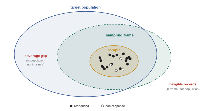
Bias enters wherever these differ. Selection bias occurs when the frame or the collection process favours some groups: a model trained on app users underrepresents people without smartphones. Non-response bias occurs when those who respond differ from those who do not. Survivorship bias occurs when only the survivors of some process are observed, such as loans that were approved (the outcomes of rejected applications are never seen). Measurement bias occurs when the recorded value systematically differs from the true value for some groups, such as a sensor that reads high in cold weather. Finally, the world changes: data collected last year may not represent next year, a problem revisited as drift in AI-410.

Simple and stratified sampling

When the data set is too large to label or process in full, a sample is drawn. A simple random sample gives every record the same chance. A stratified sample first divides records into groups (strata) and samples within each, guaranteeing that small groups are represented. Sampling the same fraction from each stratum (proportional allocation) preserves the overall mix; sampling a fixed number from each (equal allocation) oversamples small groups, which then need weights to estimate population quantities.

import numpy as np
import pandas as pd

rng = np.random.default_rng(7)
n = 100_000
region = rng.choice(["north", "south", "east", "west", "island"], size=n,
                    p=[0.40, 0.30, 0.15, 0.13, 0.02])
df = pd.DataFrame({"region": region})

simple = df.sample(n=500, random_state=1)
stratified = df.groupby("region").sample(frac=500 / n, random_state=1)

summary = pd.DataFrame({
    "population": df["region"].value_counts(normalize=True),
    "simple": simple["region"].value_counts(normalize=True),
    "stratified": stratified["region"].value_counts(normalize=True),
}).round(3)
print(summary.sort_values("population", ascending=False))
print("island rows: simple", (simple.region == "island").sum(),
      "| stratified", (stratified.region == "island").sum())

        population  simple  stratified
region
north         0.40   0.378        0.40
south         0.30   0.342        0.30
east          0.15   0.164        0.15
west          0.13   0.100        0.13
island        0.02   0.016        0.02
island rows: simple 8 | stratified 10

The stratified sample reproduces each region's share almost exactly; the simple sample is close for large regions but its count for the small island region varies by chance from sample to sample. If the island region matters, an equal-allocation sample with, say, 100 records per region would guarantee enough examples to study it.

Leakage starts at collection

Data leakage occurs when information that would not be available at prediction time finds its way into the training data, making the model look far better in testing than it will be in use. Much leakage is created at collection time:

• Fields recorded after the outcome: a churn model given a "cancellation reason" field, or a hospital readmission model given the discharge diagnosis code assigned weeks later.
• Snapshots taken today of values that changed: a customer's current account balance used to predict whether they defaulted last year. The fix is point-in-time correct data, meaning each feature value as it was known at the moment the prediction would have been made.
• Duplicates and near-duplicates across splits: the same patient, user or document appearing in both training and test sets, which rewards memorization.

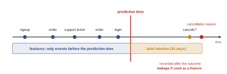
The best defence is to record, for every field, when it becomes known, and to build training examples as of a prediction time: everything before it can be a feature, and only what happens after it can be the label.

Synthetic data and augmentation

When real data is scarce, sensitive or lacks rare cases, it can be supplemented. Augmentation creates new training examples by transforming real ones, such as flipping and cropping images or paraphrasing sentences, in ways that should not change the label. Synthetic data is generated from scratch, by simulation (driving simulators, physics models) or by generative models. Both help, but neither creates information the generator lacks: a simulator that does not model sensor glare will not teach a model about glare, and a generative model trained on biased data reproduces its biases. Synthetic data should be validated by checking that models trained on it perform well on real held-out data.

How this course is organized

The course follows data from its sources to the decisions and models it supports. This lesson covers collection. Lesson 2 covers SQL for extracting data and Lesson 3 wrangling it with pandas. Lesson 4 covers cleaning and feature engineering, and Lesson 5 the special handling of text, time series, location and image data. Lesson 6 covers labelling and documenting data sets, and Lesson 7 governance, privacy and security. Lessons 8 and 9 cover pipelines and storage, and processing data at scale. Lesson 10 covers visualization and communication, Lesson 11 metrics, dashboards and experiments, and Lesson 12 the data practices that keep models working in production, ending with a complete project.