
AI-220 · Lesson 2 of 12 · 33 min
SQL for data work
Most of the data an AI practitioner uses lives in relational databases and data warehouses, and the language for getting it out is SQL. Lesson 1 showed how to read files and APIs; this lesson covers the queries that do most of the work of turning operational tables into training sets and analyses: filtering, joining, grouping, window functions and common table expressions. It also covers the mistakes that quietly corrupt results, especially joins that multiply rows and the strange logic of missing values. The examples use SQLite, which ships with Python, but the SQL is standard and runs with small changes on PostgreSQL, MySQL, BigQuery, Snowflake and other systems.
Tables, keys and the shape of a query
A relational database stores data in tables of rows and columns. Each table should have a primary key, a column (or set of columns) whose value is unique for every row, and tables refer to each other through foreign keys: an orders table has a customer_id column holding the primary key of a row in the customers table. Knowing the keys tells you the grain of each table, what one row represents (one order, one customer, one customer per day), and getting the grain right is the basis of every correct query.
A query is written in one order but logically evaluated in another:
| Step | Clause | What it does |
|---|---|---|
| 1 | FROM and JOIN | Choose the tables and combine their rows |
| 2 | WHERE | Keep rows that meet a condition |
| 3 | GROUP BY | Collapse rows into groups |
| 4 | HAVING | Keep groups that meet a condition |
| 5 | SELECT | Compute output columns, including window functions |
| 6 | ORDER BY and LIMIT | Sort and truncate the result |
This order explains common errors: a column alias defined in SELECT cannot be used in WHERE (in most databases), because WHERE is evaluated first, and a condition on an aggregate such as SUM(amount) belongs in HAVING, not WHERE.
import sqlite3

con = sqlite3.connect(":memory:")
con.executescript("""
CREATE TABLE customers (id INTEGER PRIMARY KEY, name TEXT, province TEXT);
CREATE TABLE orders (id INTEGER PRIMARY KEY, customer_id INTEGER, day TEXT, amount REAL);
""")
con.executemany("INSERT INTO customers VALUES (?, ?, ?)",
                [(1, "Amira", "ON"), (2, "Ben", "BC"), (3, "Chloe", "ON"), (4, "Dev", "AB")])
con.executemany("INSERT INTO orders VALUES (?, ?, ?, ?)",
                [(1, 1, "2026-03-02", 120.0), (2, 1, "2026-03-15", 80.0), (3, 2, "2026-03-03", 45.5),
                 (4, 3, "2026-03-09", 300.0), (5, 3, "2026-04-01", 60.0), (6, 3, "2026-04-20", 75.0),
                 (7, 9, "2026-04-22", 50.0)])

def show(sql, params=()):
    cur = con.execute(sql, params)
    print([d[0] for d in cur.description])
    for row in cur.fetchall():
        print(row)
    print()

# Filter, group and aggregate; HAVING filters groups after aggregation
show("""
SELECT c.province, COUNT(*) AS n_orders, SUM(o.amount) AS revenue
FROM orders o JOIN customers c ON c.id = o.customer_id
WHERE o.day >= ?
GROUP BY c.province
HAVING SUM(o.amount) > 100
ORDER BY revenue DESC
""", ("2026-03-01",))

# LEFT JOIN keeps customers with no orders; COALESCE turns NULL into 0
show("""
SELECT c.name, COUNT(o.id) AS n_orders, COALESCE(SUM(o.amount), 0) AS spent
FROM customers c LEFT JOIN orders o ON o.customer_id = c.id
GROUP BY c.id ORDER BY spent DESC
""")

# Orders whose customer does not exist: an orphan row
show("""
SELECT o.* FROM orders o LEFT JOIN customers c ON c.id = o.customer_id
WHERE c.id IS NULL
""")['province', 'n_orders', 'revenue']
('ON', 5, 635.0)
['name', 'n_orders', 'spent']
('Chloe', 3, 435.0)
('Amira', 2, 200.0)
('Ben', 1, 45.5)
('Dev', 0, 0)
['id', 'customer_id', 'day', 'amount']
(7, 9, '2026-04-22', 50.0)Three details in this example matter in practice. Values are passed as parameters (the ? placeholders) rather than pasted into the SQL string, which prevents SQL injection and handles quoting correctly. The LEFT JOIN keeps Dev, who has no orders, with COUNT(o.id) giving 0 because COUNT of a column ignores missing values. And the last query finds an order whose customer does not exist, a referential-integrity problem that an inner join would silently drop.
Joins
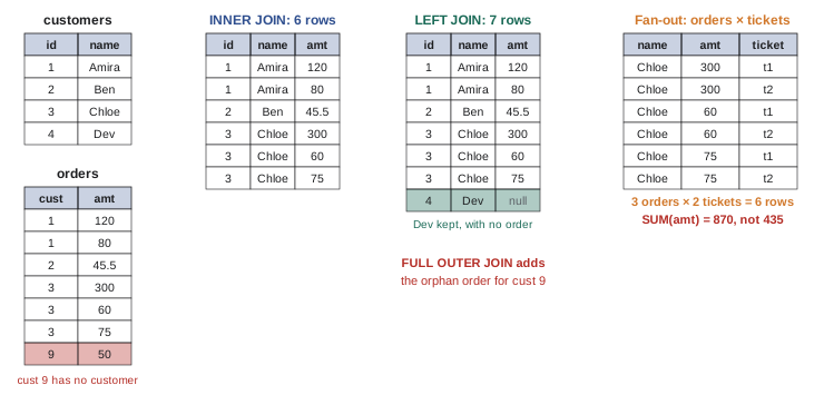
A join combines rows of two tables that satisfy a condition, usually equality of keys:
- INNER JOIN keeps only pairs of rows that match.
- LEFT JOIN keeps every row of the left table, with missing values (NULL) where there is no match on the right.
- FULL OUTER JOIN keeps unmatched rows from both sides.
- CROSS JOIN pairs every row with every row, useful for building grids such as every customer for every month.
Fan-out: the most common silent error
When a customer has three orders and two support tickets, joining customers to both orders and tickets produces 3 × 2 = 6 rows for that customer. Summing order amounts over those rows counts each order twice. No error is raised; the totals are simply wrong.
import sqlite3

con = sqlite3.connect(":memory:")
con.executescript("""
CREATE TABLE customers (id INTEGER PRIMARY KEY, name TEXT, province TEXT);
CREATE TABLE orders (id INTEGER PRIMARY KEY, customer_id INTEGER, day TEXT, amount REAL);
""")
con.executemany("INSERT INTO customers VALUES (?, ?, ?)",
                [(1, "Amira", "ON"), (2, "Ben", "BC"), (3, "Chloe", "ON"), (4, "Dev", "AB")])
con.executemany("INSERT INTO orders VALUES (?, ?, ?, ?)",
                [(1, 1, "2026-03-02", 120.0), (2, 1, "2026-03-15", 80.0), (3, 2, "2026-03-03", 45.5),
                 (4, 3, "2026-03-09", 300.0), (5, 3, "2026-04-01", 60.0), (6, 3, "2026-04-20", 75.0),
                 (7, 9, "2026-04-22", 50.0)])

def show(sql, params=()):
    cur = con.execute(sql, params)
    print([d[0] for d in cur.description])
    for row in cur.fetchall():
        print(row)
    print()

# A second one-to-many table: support tickets per customer
con.execute("CREATE TABLE tickets (id INTEGER PRIMARY KEY, customer_id INTEGER)")
con.executemany("INSERT INTO tickets VALUES (?, ?)", [(1, 3), (2, 3), (3, 1)])

# Wrong: joining two one-to-many tables multiplies rows (fan-out)
show("""
SELECT c.name, SUM(o.amount) AS revenue, COUNT(t.id) AS tickets
FROM customers c
JOIN orders o ON o.customer_id = c.id
LEFT JOIN tickets t ON t.customer_id = c.id
GROUP BY c.id ORDER BY c.id
""")

# Right: aggregate each table to one row per customer first, then join
show("""
WITH rev AS (SELECT customer_id, SUM(amount) AS revenue FROM orders GROUP BY customer_id),
     tix AS (SELECT customer_id, COUNT(*) AS tickets FROM tickets GROUP BY customer_id)
SELECT c.name, rev.revenue, COALESCE(tix.tickets, 0) AS tickets
FROM customers c
JOIN rev ON rev.customer_id = c.id
LEFT JOIN tix ON tix.customer_id = c.id
ORDER BY c.id
""")['name', 'revenue', 'tickets']
('Amira', 200.0, 2)
('Ben', 45.5, 0)
('Chloe', 870.0, 6)
['name', 'revenue', 'tickets']
('Amira', 200.0, 1)
('Ben', 45.5, 0)
('Chloe', 435.0, 2)The defence is to know the grain of every table and to check row counts: before and after each join, count rows and distinct keys. If a join is supposed to keep one row per customer, the result should have exactly as many rows as there are customers. Aggregating to the target grain before joining, as in the corrected query, is the standard fix.
Worked problem
Predicting a row count
A table of 10,000 patients joins to visits (average 4.2 per patient) and to prescriptions (average 2.5 per patient), both by patient id, with inner joins. Assuming every patient has at least one of each and counts are independent, about how many rows result, and what happens to a SUM of visit costs?
Show solution
- Each patient contributes (visits × prescriptions) rows; on average roughly \(4.2 \times 2.5 = 10.5\).
- Total: about \(10{,}000 \times 10.5 = 105{,}000\) rows.
- Each visit cost appears once for every prescription of that patient, so the SUM is inflated by the prescription count, about 2.5 times on average.
Answer: About 105,000 rows, and total visit cost inflated by roughly 2.5 times. Aggregate visits and prescriptions separately to one row per patient, then join.
Grouping and aggregation
GROUP BY collapses rows sharing the same values into one row per group, and aggregate functions summarize each group: COUNT, SUM, AVG, MIN, MAX, and in many databases statistical functions such as percentiles and standard deviations. Every column in SELECT must either be in the GROUP BY or be inside an aggregate; SQLite and MySQL in some modes accept other columns and pick an arbitrary value, which is a source of subtle bugs.
For feature engineering, grouping turns event tables into one row per entity: the number of orders per customer in the last 90 days, the mean and maximum of a sensor per machine per hour, the share of a user's sessions on mobile. The time window must end at the prediction time for each example, or the features leak future information (Lesson 1).
Window functions
A window function computes a value over a set of rows related to the current row, without collapsing them. The OVER clause defines the window: PARTITION BY splits rows into groups, ORDER BY orders them within each group, and an optional frame (such as ROWS BETWEEN 6 PRECEDING AND CURRENT ROW) limits which rows are included. Window functions are ideal for:
- Running totals and moving averages.
- Ranking: ROW_NUMBER, RANK and DENSE_RANK, for example to pick the latest or largest row per group.
- Comparing with neighbouring rows: LAG and LEAD give the previous and next values, for changes and time between events.
- Shares of a total: dividing by SUM(...) OVER () with an empty window covering all rows.
import sqlite3

con = sqlite3.connect(":memory:")
con.executescript("""
CREATE TABLE customers (id INTEGER PRIMARY KEY, name TEXT, province TEXT);
CREATE TABLE orders (id INTEGER PRIMARY KEY, customer_id INTEGER, day TEXT, amount REAL);
""")
con.executemany("INSERT INTO customers VALUES (?, ?, ?)",
                [(1, "Amira", "ON"), (2, "Ben", "BC"), (3, "Chloe", "ON"), (4, "Dev", "AB")])
con.executemany("INSERT INTO orders VALUES (?, ?, ?, ?)",
                [(1, 1, "2026-03-02", 120.0), (2, 1, "2026-03-15", 80.0), (3, 2, "2026-03-03", 45.5),
                 (4, 3, "2026-03-09", 300.0), (5, 3, "2026-04-01", 60.0), (6, 3, "2026-04-20", 75.0),
                 (7, 9, "2026-04-22", 50.0)])

def show(sql, params=()):
    cur = con.execute(sql, params)
    print([d[0] for d in cur.description])
    for row in cur.fetchall():
        print(row)
    print()

# Window functions keep every row while computing over a group of rows
show("""
SELECT customer_id, day, amount,
       SUM(amount) OVER (PARTITION BY customer_id ORDER BY day) AS running_total,
       ROW_NUMBER() OVER (PARTITION BY customer_id ORDER BY day) AS order_no,
       amount - LAG(amount) OVER (PARTITION BY customer_id ORDER BY day) AS change
FROM orders WHERE customer_id IN (1, 3)
ORDER BY customer_id, day
""")

# Latest order per customer: rank inside a CTE, then keep rank 1
show("""
WITH ranked AS (
  SELECT o.*, ROW_NUMBER() OVER (PARTITION BY customer_id ORDER BY day DESC) AS rk
  FROM orders o)
SELECT customer_id, day, amount FROM ranked WHERE rk = 1 ORDER BY customer_id
""")

# Monthly revenue and share of the total
show("""
SELECT substr(day, 1, 7) AS month, SUM(amount) AS revenue,
       ROUND(100.0 * SUM(amount) / SUM(SUM(amount)) OVER (), 1) AS pct
FROM orders GROUP BY month ORDER BY month
""")['customer_id', 'day', 'amount', 'running_total', 'order_no', 'change']
(1, '2026-03-02', 120.0, 120.0, 1, None)
(1, '2026-03-15', 80.0, 200.0, 2, -40.0)
(3, '2026-03-09', 300.0, 300.0, 1, None)
(3, '2026-04-01', 60.0, 360.0, 2, -240.0)
(3, '2026-04-20', 75.0, 435.0, 3, 15.0)
['customer_id', 'day', 'amount']
(1, '2026-03-15', 80.0)
(2, '2026-03-03', 45.5)
(3, '2026-04-20', 75.0)
(9, '2026-04-22', 50.0)
['month', 'revenue', 'pct']
('2026-03', 545.5, 74.7)
('2026-04', 185.0, 25.3)The second query uses a common table expression (CTE), introduced by WITH, which names an intermediate result so the query reads top to bottom as a series of steps. CTEs replace deeply nested subqueries and make complex transformations reviewable.
Worked problem
A seven-day moving average
Write the window expression for a seven-day moving average of daily_sales in a table with one row per store per day, and say what it returns for the first day of each store.
Show solution
- Window: AVG(daily_sales) OVER (PARTITION BY store_id ORDER BY day ROWS BETWEEN 6 PRECEDING AND CURRENT ROW).
- On a store's first day, only one row is in the frame, so it returns that day's value.
Answer: The expression above. Early values average fewer than seven days, and missing days are not counted as zero: if the table skips days, ROWS counts rows, not calendar days. Fill missing days first (with a calendar table and a LEFT JOIN) or use a RANGE frame on dates where the database supports it.
Missing values: NULL and three-valued logic
SQL represents a missing value as NULL, and NULL behaves unlike any other value. Any comparison with NULL, even NULL = NULL, gives NULL (unknown), not true or false, and WHERE keeps only rows where the condition is true. This three-valued logic produces surprising results:
import sqlite3

con = sqlite3.connect(":memory:")
con.execute("CREATE TABLE t (id INTEGER, score REAL)")
con.executemany("INSERT INTO t VALUES (?, ?)", [(1, 10.0), (2, None), (3, 30.0), (4, None)])

def one(sql):
    return con.execute(sql).fetchall()

print("NULL = NULL      ->", one("SELECT NULL = NULL"))
print("rows score > 5   ->", one("SELECT COUNT(*) FROM t WHERE score > 5"))
print("rows NOT > 5     ->", one("SELECT COUNT(*) FROM t WHERE NOT (score > 5)"))
print("COUNT(*), COUNT(score) ->", one("SELECT COUNT(*), COUNT(score) FROM t"))
print("AVG(score)       ->", one("SELECT AVG(score) FROM t"))
print("AVG with 0 for NULL ->", one("SELECT AVG(COALESCE(score, 0)) FROM t"))

# NOT IN with a NULL in the list matches nothing
con.execute("CREATE TABLE banned (id INTEGER)")
con.executemany("INSERT INTO banned VALUES (?)", [(2,), (None,)])
print("NOT IN           ->", one("SELECT id FROM t WHERE id NOT IN (SELECT id FROM banned)"))
print("NOT EXISTS       ->", one("""SELECT id FROM t WHERE NOT EXISTS
(SELECT 1 FROM banned b WHERE b.id = t.id)"""))NULL = NULL -> [(None,)] rows score > 5 -> [(2,)] rows NOT > 5 -> [(0,)] COUNT(*), COUNT(score) -> [(4, 2)] AVG(score) -> [(20.0,)] AVG with 0 for NULL -> [(10.0,)] NOT IN -> [] NOT EXISTS -> [(1,), (3,), (4,)]
Key lessons from the output:
- A row with a NULL score passes neither score > 5 nor NOT (score > 5); test explicitly with IS NULL.
- COUNT(*) counts rows; COUNT(column) counts non-null values. AVG ignores NULLs, which may or may not be what you want: treating missing as zero gives a different answer.
- NOT IN against a subquery that contains a NULL returns no rows at all. Use NOT EXISTS, which behaves as expected.
From queries to training sets
A typical extraction for a model builds one row per example with features computed as of a cut-off time and a label from after it:
- A spine query lists the examples: entity ids and their prediction times.
- Feature CTEs aggregate each event table, filtered to events before each example's prediction time, to one row per example.
- A label CTE computes the outcome in the window after the prediction time.
- The final SELECT left-joins features and labels to the spine, so that examples with no events still appear (with zero or missing features).
Row counts are checked at each step: the final table must have exactly one row per example. The query is saved in version control with the model code, so that the training set can be rebuilt and audited (Lesson 8).
Worked problem
Writing the time condition
The spine has columns customer_id and cutoff. Write the join condition that brings in orders from the 90 days before each cutoff, but not on or after it, with dates stored as ISO text.
Show solution
- Match the customer: o.customer_id = s.customer_id.
- Before the cutoff: o.day < s.cutoff.
- Within 90 days: o.day >= date(s.cutoff, '-90 days') in SQLite (or s.cutoff - INTERVAL 90 DAY in other dialects).
Answer: JOIN on all three conditions, then GROUP BY s.customer_id, s.cutoff. The strict "<" matters: an order placed on the cutoff date may not be known at prediction time.
Performance in brief
Queries on large tables can be slow or expensive, especially in cloud warehouses that charge by data scanned. A few habits help:
- Select only the columns you need; columnar warehouses read only those columns.
- Filter early, especially on partition columns such as dates, so the engine can skip data.
- Use indexes on join and filter columns in transactional databases; inspect the query plan (EXPLAIN) when a query is slow.
- Aggregate before joining large tables, which is both faster and avoids fan-out.
- Develop on a sample, using LIMIT or a filtered date range, and run on the full data once the logic is right.
Common mistakes
MistakeJoining two one-to-many tables to the same key and summing.
InsteadAggregate each table to the target grain first, then join; check row counts.
MistakePasting values into SQL strings.
InsteadPass values as parameters to avoid injection and quoting errors.
MistakeUsing NOT IN with a subquery that may contain NULL.
InsteadUse NOT EXISTS.
MistakePutting conditions on aggregates in WHERE.
InsteadUse HAVING for conditions on groups.
MistakeUsing an inner join when examples may have no events.
InsteadLeft-join features to a spine so every example appears.
Summary and key terms
- Know each table's grain and keys; queries are evaluated FROM, WHERE, GROUP BY, HAVING, SELECT, ORDER BY.
- Inner, left, full and cross joins combine tables; fan-out multiplies rows silently.
- GROUP BY with aggregates builds one row per entity; HAVING filters groups.
- Window functions give running totals, rankings, lags and shares without collapsing rows.
- NULL makes comparisons unknown; COUNT and AVG skip NULLs; NOT IN fails with NULLs.
- Training sets come from a spine, time-bounded feature CTEs and a label, with row-count checks.
- Primary key
- A column or set of columns unique for every row.
- Foreign key
- A column holding the primary key of a row in another table.
- Grain
- What one row of a table represents.
- Inner join
- A join keeping only matching pairs of rows.
- Left join
- A join keeping all rows of the left table.
- Fan-out
- Row multiplication from joining one-to-many relationships.
- Window function
- A calculation over related rows that keeps every row.
- CTE
- A common table expression: a named intermediate result introduced by WITH.
- NULL
- SQL's marker for a missing value.
- Spine
- The table listing examples and their prediction times.
Practice problems
Work each problem on paper first, then reveal the answer to check.
In which clause does a condition on SUM(amount) belong?
Show answer
HAVING.
Why can a SELECT alias not be used in WHERE?
Show answer
WHERE is evaluated before SELECT.
A customer has 4 orders and 3 tickets. Rows after joining both?
Show answer
12.
What does COUNT(o.id) give for a customer with no orders in a LEFT JOIN?
Show answer
0.
Which function picks the latest row per group?
Show answer
ROW_NUMBER() ordered by date descending, keeping rank 1.
What does LAG(x) return on the first row of a partition?
Show answer
NULL.
Result of NULL = NULL?
Show answer
NULL (unknown).
AVG of 10, NULL, 30?
Show answer
20.
Why prefer NOT EXISTS to NOT IN?
Show answer
NOT IN returns nothing if the subquery contains a NULL.
What check confirms a training-set query is correct at the end?
Show answer
Exactly one row per example in the spine.
Lesson quiz · 5 questions
Score 60% or more to complete this lesson.
Create a free account to save your progress, take quizzes and earn a certificate.