Metrics, dashboards and experiments

Lesson 10 covered how to make individual charts honest and clear. Much of the data work in organizations, however, goes into recurring products: metrics that track how a product, process or model is doing, dashboards that display them, and experiments that test whether a change made things better. Each has characteristic traps. A metric can be defined in two reasonable ways that disagree; a dashboard can show many numbers and answer no question; an experiment can declare a winner that is noise. This lesson covers how to define metrics precisely, how to design dashboards that support decisions, the paradoxes of aggregated data, and the statistics and practice of A/B testing.

Defining a metric

A metric is a number computed the same way every time, so that changes in it reflect changes in the world rather than in the calculation. A good metric definition states:

• The numerator and denominator, with exact inclusion rules (which events, which users, which statuses).
• The unit of analysis: per user, per session, per order, per day.
• The time window and time zone.
• How missing data, test accounts, bots, refunds and duplicates are handled.
• The owner, and where the calculation lives (one shared definition in code or a metrics layer, not reimplemented in each dashboard).

Ratio metrics

Many metrics are ratios: conversion rate, click-through rate, error rate. A ratio can be computed as the mean of per-unit ratios or as the ratio of totals, and the two answer different questions.

import pandas as pd

# Sessions and conversions per user for one week
users = pd.DataFrame({
    "user": ["a", "b", "c", "d", "e"],
    "sessions": [1, 1, 2, 40, 6],
    "orders": [1, 0, 1, 4, 0],
})
users["rate"] = users["orders"] / users["sessions"]

mean_of_ratios = users["rate"].mean()
ratio_of_sums = users["orders"].sum() / users["sessions"].sum()
print(users.to_string(index=False))
print(f"mean of per-user rates : {mean_of_ratios:.3f}  (each user counts equally)")
print(f"total orders / sessions: {ratio_of_sums:.3f}  (each session counts equally)")

user  sessions  orders  rate
   a         1       1   1.0
   b         1       0   0.0
   c         2       1   0.5
   d        40       4   0.1
   e         6       0   0.0
mean of per-user rates : 0.320  (each user counts equally)
total orders / sessions: 0.120  (each session counts equally)

The mean of ratios weights every user equally, which suits questions about the typical user. The ratio of totals weights every session equally, which suits questions about the business as a whole. Neither is wrong, but a metric must say which it is, and the two should never be compared with each other.

Leading, lagging and guardrail metrics

Organizations usually track a small hierarchy of metrics:

• A north-star or primary metric that reflects the value delivered, such as weekly active customers who complete a purchase.
• Leading indicators that move sooner and predict it, such as sign-ups or first-week engagement.
• Guardrail metrics that must not get worse, such as latency, error rates, complaints, refunds, and fairness measures across groups.

Any metric that becomes a target can be gamed, consciously or not (Goodhart's law): a support team measured on ticket closure time may close tickets prematurely. Guardrails and periodic review of what a metric actually rewards are the defences.

Simpson's paradox

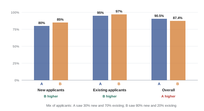
Aggregating across groups can reverse a relationship that holds within every group. This is Simpson's paradox, and it appears whenever the groups differ in size between the things being compared and also differ in their rates.

import pandas as pd

# Approval rates for two models, by applicant segment
rows = [
    ("model A", "new", 300, 240), ("model A", "existing", 700, 665),
    ("model B", "new", 800, 680), ("model B", "existing", 200, 194),
]
df = pd.DataFrame(rows, columns=["model", "segment", "applicants", "approved"])
df["rate"] = (df["approved"] / df["applicants"]).round(3)
print(df.pivot(index="segment", columns="model", values="rate"))

overall = df.groupby("model")[["applicants", "approved"]].sum()
overall["rate"] = (overall["approved"] / overall["applicants"]).round(3)
print(overall)

model     model A  model B
segment
existing     0.95     0.97
new          0.80     0.85
         applicants  approved   rate
model
model A        1000       905  0.905
model B        1000       874  0.874

Model B is better within each segment, but most of its applicants were new customers, who have lower approval rates whatever the model; model A saw mostly existing customers. The overall comparison mixes the effect of the model with the effect of the mix. When groups differ in composition, compare within groups, or adjust for the composition (standardize to a common mix), and ask which comparison answers the decision at hand. Randomized experiments avoid the problem by making the groups alike.

Dashboards that support decisions

A dashboard is a set of charts and numbers that people check repeatedly. Good dashboards are designed backwards from the decisions they support:

• Purpose: who uses it, how often, and what they will do when a number changes. A dashboard for an operations team watching a data centre every minute differs from a monthly executive summary.
• Hierarchy: the few most important numbers at the top, with context (target, previous period, trend), and detail below for diagnosis.
• Comparisons: every number shown with something to compare it to, such as last week, the same week last year, a target or a forecast range. A number on its own cannot be judged.
• Consistency: shared metric definitions, the same time zone and period across charts, the same colours for the same categories.
• Freshness and quality: when the data was last updated, and a visible warning when a pipeline is late or a data quality check has failed (Lesson 8).
• Restraint: fewer charts, each answering a question. Dashboards accumulate charts that nobody uses; review and remove them.

A/B testing

The most reliable way to learn whether a change causes an improvement is a randomized controlled experiment, called an A/B test in product and model work. Users (or sessions, stores, regions) are randomly assigned to control (A) or treatment (B), and the metric is compared. Randomization makes the groups alike in everything except the change, on average, so a difference beyond what chance explains can be attributed to the change.

Steps in a well-run test:

• State the hypothesis, the primary metric, guardrails, and the minimum effect worth detecting, before starting.
• Calculate the sample size needed, and the duration, including whole weeks to cover weekly cycles.
• Randomize at the right unit: if users see the change across sessions, randomize by user, and analyse by user.
• Check the split: the share of units in each group should match the design (a sample ratio mismatch signals a bug).
• Run for the planned duration, then analyse once.

import math
from scipy.stats import norm

# A/B test of a checkout change: conversions out of visitors
n_a, x_a = 24_000, 1_152      # control
n_b, x_b = 24_000, 1_272      # treatment
p_a, p_b = x_a / n_a, x_b / n_b
p = (x_a + x_b) / (n_a + n_b)
se0 = math.sqrt(p * (1 - p) * (1 / n_a + 1 / n_b))
z = (p_b - p_a) / se0
p_value = 2 * (1 - norm.cdf(abs(z)))
se = math.sqrt(p_a * (1 - p_a) / n_a + p_b * (1 - p_b) / n_b)
lo, hi = (p_b - p_a) - 1.96 * se, (p_b - p_a) + 1.96 * se
print(f"control {p_a:.4f}, treatment {p_b:.4f}, lift {100 * (p_b / p_a - 1):.1f}%")
print(f"z = {z:.2f}, p = {p_value:.4f}, 95% CI for difference [{lo:.4f}, {hi:.4f}]")

# Sample size per group to detect a 0.5 point change from 4.8% with 80% power
def n_per_group(p0, delta, alpha=0.05, power=0.8):
    za, zb = norm.ppf(1 - alpha / 2), norm.ppf(power)
    p1 = p0 + delta
    return math.ceil((za + zb) ** 2 * (p0 * (1 - p0) + p1 * (1 - p1)) / delta ** 2)

for delta in (0.010, 0.005, 0.0025):
    print(f"detect +{100 * delta:.2f} points: {n_per_group(0.048, delta):,} per group")

control 0.0480, treatment 0.0530, lift 10.4%
z = 2.50, p = 0.0124, 95% CI for difference [0.0011, 0.0089]
detect +1.00 points: 7,875 per group
detect +0.50 points: 30,105 per group
detect +0.25 points: 117,603 per group

The test found a 0.5 point increase in conversion (a 10.4% relative lift), with a 95% confidence interval from 0.11 to 0.89 points: the change very likely helps, but the true size of the effect is uncertain by a factor of eight. The sample-size calculation shows the cost of detecting small effects: halving the detectable effect roughly quadruples the users needed, because the standard error falls only with the square root of the sample size.

Peeking and other pitfalls

The most common error in practice is checking results every day and stopping as soon as the difference looks significant. Each look is another chance for noise to cross the threshold, so the real false-positive rate is far above the nominal 5%.

import numpy as np
from scipy.stats import norm

# A/A tests: both groups identical, so every "significant" result is a false positive
rng = np.random.default_rng(11)
experiments, days, per_day, p = 2000, 20, 500, 0.05
peek_hits = final_hits = 0
for _ in range(experiments):
    a = rng.binomial(per_day, p, days).cumsum()
    b = rng.binomial(per_day, p, days).cumsum()
    n = per_day * np.arange(1, days + 1)
    pooled = (a + b) / (2 * n)
    z = (b - a) / n / np.sqrt(pooled * (1 - pooled) * 2 / n)
    sig = np.abs(z) > norm.ppf(0.975)
    peek_hits += sig.any()          # stop at the first day that looks significant
    final_hits += sig[-1]           # test once, at the planned end
print(f"false positive rate, test once at the end: {final_hits / experiments:.3f}")
print(f"false positive rate, peek every day      : {peek_hits / experiments:.3f}")

false positive rate, test once at the end: 0.045
false positive rate, peek every day      : 0.236

Solutions are to fix the duration in advance and analyse once, or to use methods designed for continuous monitoring, such as sequential tests with adjusted thresholds or always-valid confidence intervals, which many experimentation platforms provide. Other pitfalls:

• Many metrics and segments: testing 20 metrics at 5% will usually find one "significant" by chance. Name one primary metric and correct for multiple comparisons when exploring.
• Novelty and learning effects: users react to anything new at first; effects can fade or grow over weeks.
• Interference: when units affect each other (a ride-sharing market, a social network, shared inventory), treatment spills into control, and randomization by region or time is needed.
• Practical significance: a statistically significant effect may be too small to matter, and a large effect may be uncertain. Report the effect size and its interval, not only the p-value.

Testing models

A new machine learning model is evaluated offline on held-out data (Lesson 6 covered honest splits), but offline metrics do not always predict business outcomes. Online A/B tests compare models on the real metric, with guardrails on latency, errors and fairness. Shadow deployment, running the new model alongside the old without acting on its output, is a lower-risk step before an A/B test, and catches errors in features and serving (Lesson 12).