Wrangling data with pandas

Once data has been extracted, most of the work of preparing it happens in a dataframe library, and in Python that usually means pandas. Wrangling is the reshaping, combining and summarizing that turns raw tables into the form an analysis or model needs. Done carelessly it introduces errors that are hard to see: rows multiplied by a merge, values aligned to the wrong dates, groups computed across the wrong boundaries. This lesson covers tidy data and reshaping, grouped operations, merges that check their own assumptions, and the handling of dates, times and time zones, including joins that respect the moment each fact became known.

Tidy data

Data is tidy when each variable is a column, each observation is a row, and each type of observation is a table. Many sources are not tidy: spreadsheets often put years or months across the columns, survey exports put each answer option in its own column, and sensor exports put several measurements in one text field. Tidy data is easier to filter, group, plot and model, because every operation can refer to variables by name.

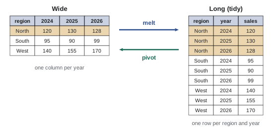
The two basic reshaping operations are:

• melt (wide to long): turn several columns into two, one naming the former column (the year, say) and one holding its value.
• pivot (long to wide): spread one column's values across new columns, for reports or for models that expect one column per feature.

import pandas as pd

# Wide: one column per year, as often found in spreadsheets
wide = pd.DataFrame({
    "region": ["North", "South", "West"],
    "2024": [120, 95, 140],
    "2025": [130, 90, 155],
    "2026": [128, 99, 170],
})
long = wide.melt(id_vars="region", var_name="year", value_name="sales")
long["year"] = long["year"].astype(int)
print(long.sort_values(["region", "year"]).to_string(index=False))

# Long data is easy to group and model
growth = long.sort_values("year").groupby("region")["sales"].agg(["first", "last"])
growth["pct"] = (100 * (growth["last"] / growth["first"] - 1)).round(1)
print(growth)

# And easy to turn back into a report table
print(long.pivot(index="year", columns="region", values="sales"))

region  year  sales
 North  2024    120
 North  2025    130
 North  2026    128
 South  2024     95
 South  2025     90
 South  2026     99
  West  2024    140
  West  2025    155
  West  2026    170
        first  last   pct
region
North     120   128   6.7
South      95    99   4.2
West      140   170  21.4
region  North  South  West
year
2024      120     95   140
2025      130     90   155
2026      128     99   170

In the long form, the year is an ordinary variable that can be sorted, filtered and used as a feature, and a new year adds rows rather than a column, so code does not have to change when data grows.

Split, apply, combine

Grouped operations follow a pattern: split the data into groups by one or more keys, apply a function to each group, and combine the results. pandas offers three kinds of apply:

• agg: reduce each group to one row (count, sum, mean, quantiles). Named aggregation gives the output columns clear names.
• transform: compute a group statistic and broadcast it back to every row of the group, keeping the original shape. This is how to express each row relative to its group: share of the group total, difference from the group mean, rank within the group.
• filter: keep or drop whole groups based on a condition.

import numpy as np
import pandas as pd

rng = np.random.default_rng(3)
df = pd.DataFrame({
    "store": rng.choice(["A", "B", "C"], 12),
    "product": rng.choice(["tea", "coffee"], 12),
    "units": rng.integers(1, 20, 12),
    "price": rng.choice([3.5, 4.0, 4.5], 12),
})
df["revenue"] = df["units"] * df["price"]

# agg: one row per group, with named outputs
summary = df.groupby("store").agg(
    orders=("units", "size"),
    units=("units", "sum"),
    revenue=("revenue", "sum"),
    avg_price=("price", "mean"),
).round(2)
print(summary)

# transform: a group statistic broadcast back to every row
df["store_share"] = (df["revenue"] / df.groupby("store")["revenue"].transform("sum")).round(3)
df["units_vs_store_mean"] = df["units"] - df.groupby("store")["units"].transform("mean").round(1)
print(df.head(5).to_string(index=False))

# filter: keep only groups that meet a condition
big = df.groupby("store").filter(lambda g: g["revenue"].sum() > 150)
print("stores kept:", sorted(big["store"].unique()))

       orders  units  revenue  avg_price
store
A           7     66    272.0       4.07
B           2     32    131.0       4.00
C           3     38    137.0       3.67
store product  units  price  revenue  store_share  units_vs_store_mean
    C  coffee      8    4.0     32.0        0.234                 -4.7
    A     tea      9    4.5     40.5        0.149                 -0.4
    A     tea     13    4.5     58.5        0.215                  3.6
    A     tea     12    3.5     42.0        0.154                  2.6
    A  coffee      4    4.5     18.0        0.066                 -5.4
stores kept: ['A']

Group-relative features, like those made with transform, are among the most useful in practice: a transaction that is large for this customer, a reading that is high for this machine, a price that is low for this neighbourhood. They must be computed using only training data (and only data before each example's prediction time), or they leak information into evaluation (Lesson 4).

Merging with checks

A merge (join) in pandas has the same semantics as in SQL (Lesson 2), and the same dangers. The most common error is a duplicated key on the side that is supposed to be unique: each duplicate creates an extra copy of the matching rows on the other side, inflating counts and sums without any warning. Two arguments turn hidden assumptions into checks:

• validate states the expected relationship, "one_to_one", "one_to_many" or "many_to_one", and raises an error if the keys do not satisfy it.
• indicator adds a column showing whether each row matched on both sides or only one, so unmatched rows can be counted and investigated.

import pandas as pd

customers = pd.DataFrame({"cust": [1, 2, 3, 3], "segment": ["retail", "retail", "business", "business"]})
orders = pd.DataFrame({"order": [10, 11, 12, 13], "cust": [1, 3, 3, 4], "amount": [50, 70, 30, 20]})

# A duplicated key on the "one" side silently creates extra rows
m = orders.merge(customers, on="cust", how="left")
print("rows before", len(orders), "after", len(m))

# validate= turns that silent error into an exception
try:
    orders.merge(customers, on="cust", how="left", validate="many_to_one")
except pd.errors.MergeError as e:
    print("MergeError:", str(e).splitlines()[0])

# Fix the duplicate, then merge with an indicator to see unmatched rows
customers = customers.drop_duplicates("cust")
m = orders.merge(customers, on="cust", how="left", validate="many_to_one", indicator=True)
print(m.to_string(index=False))
print(m["_merge"].value_counts().to_dict())

rows before 4 after 6
MergeError: Merge keys are not unique in right dataset; not a many-to-one merge
 order  cust  amount  segment    _merge
    10     1      50   retail      both
    11     3      70 business      both
    12     3      30 business      both
    13     4      20      NaN left_only
{'both': 3, 'left_only': 1, 'right_only': 0}

A good habit is to state the expected row count after every merge and assert it in code. A merge of orders to customers with how="left" and validate="many_to_one" must return exactly as many rows as there are orders; if it does not, something is wrong with the keys.

Keys that look equal but are not

Merges fail to match when keys differ in type or format: an integer 42 and a string "42", "A-001" and "a-001", trailing spaces, leading zeros dropped by a spreadsheet (postal codes, product codes). Normalize keys before merging, and check the match rate with the indicator.

Dates, times and time zones

Time is the most error-prone kind of data. A timestamp without a time zone is ambiguous; a local time around a daylight-saving change may occur twice or not at all; and different systems record events in different zones. Robust practice is:

• Store and compute in UTC; convert to local time only for display and for grouping by local calendar day.
• Parse timestamps with an explicit format and time zone, and check the result.
• Be aware that a local day can have 23 or 25 hours, and that "daily" aggregates depend on which day boundary is used.

import pandas as pd

# Meter readings recorded in UTC around the 2026 autumn clock change in Toronto
utc = pd.date_range("2026-10-31 22:00", periods=8, freq="2h", tz="UTC")
readings = pd.DataFrame({"time": utc, "kwh": [1.0, 1.2, 0.8, 0.7, 0.9, 1.4, 1.6, 1.5]})
readings["local"] = readings["time"].dt.tz_convert("America/Toronto")
print(readings[["time", "local", "kwh"]].to_string(index=False))

# Daily totals by LOCAL calendar day: resample after converting
daily = readings.set_index("local")["kwh"].resample("D").sum()
print(daily)

# Point-in-time join: attach the price in force at each reading
prices = pd.DataFrame({
    "time": pd.to_datetime(["2026-10-31 00:00", "2026-11-01 07:00"], utc=True),
    "price": [0.098, 0.151],
})
joined = pd.merge_asof(readings.sort_values("time"), prices.sort_values("time"),
                       on="time", direction="backward")
joined["cost"] = (joined["kwh"] * joined["price"]).round(3)
print(joined[["time", "kwh", "price", "cost"]].to_string(index=False))

                     time                     local  kwh
2026-10-31 22:00:00+00:00 2026-10-31 18:00:00-04:00  1.0
2026-11-01 00:00:00+00:00 2026-10-31 20:00:00-04:00  1.2
2026-11-01 02:00:00+00:00 2026-10-31 22:00:00-04:00  0.8
2026-11-01 04:00:00+00:00 2026-11-01 00:00:00-04:00  0.7
2026-11-01 06:00:00+00:00 2026-11-01 01:00:00-05:00  0.9
2026-11-01 08:00:00+00:00 2026-11-01 03:00:00-05:00  1.4
2026-11-01 10:00:00+00:00 2026-11-01 05:00:00-05:00  1.6
2026-11-01 12:00:00+00:00 2026-11-01 07:00:00-05:00  1.5
local
2026-10-31 00:00:00-04:00    3.0
2026-11-01 00:00:00-04:00    6.1
Freq: D, Name: kwh, dtype: float64
                     time  kwh  price  cost
2026-10-31 22:00:00+00:00  1.0  0.098 0.098
2026-11-01 00:00:00+00:00  1.2  0.098 0.118
2026-11-01 02:00:00+00:00  0.8  0.098 0.078
2026-11-01 04:00:00+00:00  0.7  0.098 0.069
2026-11-01 06:00:00+00:00  0.9  0.098 0.088
2026-11-01 08:00:00+00:00  1.4  0.151 0.211
2026-11-01 10:00:00+00:00  1.6  0.151 0.242
2026-11-01 12:00:00+00:00  1.5  0.151 0.226

The conversion shows the offset changing from −04:00 to −05:00 on 1 November: the readings are evenly spaced in UTC, but local times jump. Resampling by local day after conversion puts each reading in the right calendar day for a Toronto customer.

Point-in-time joins

The last part of the example uses merge_asof, which joins each row to the most recent row of another table at or before its timestamp. This is the right tool whenever a value changes over time and each event needs the value in force when it occurred: prices, exchange rates, a customer's plan, a model version, a sensor's calibration. An ordinary merge on date would either fail to match or attach a value that was not yet known, a subtle form of leakage.

Performance and correctness habits

pandas is fast when operations are vectorized, applied to whole columns at once, and slow when Python loops run over rows. A few habits keep code fast and correct:

• Prefer column operations, groupby and merges to loops and row-wise apply.
• Use appropriate types: categories for repeated strings, nullable integers for integer columns with missing values, datetime types for times. Lesson 9 shows how much memory this saves.
• Avoid chained assignment (setting values on a filtered copy); use .loc with a boolean mask on the original frame.
• Assert invariants: unique keys, expected row counts, no missing values in required columns, values within valid ranges.
• Keep wrangling code in functions or scripts, not only in notebook cells run out of order, so it can be re-run from raw data.