Data for machine learning in production

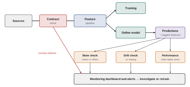
A model trained on a carefully prepared data set is only the beginning. Once deployed, it depends every day on data arriving from systems that change: a new app version renames a field, a supplier sends prices in another currency, customer behaviour shifts with the season or the economy, and the model's own decisions change the data it will later be trained on. Most production failures of machine learning systems are data failures, not modelling failures. This final lesson covers the practices that keep data reliable for models in production, data contracts, drift monitoring, training-serving consistency and feedback loops, and then walks through a complete project that uses the methods of the whole course.

Data contracts

A data contract is an explicit agreement between the team that produces a data set and the teams that consume it. It specifies the schema (column names and types), the meaning of each field, allowed values and ranges, uniqueness, freshness (how soon after events data arrives), volume expectations, and how changes will be announced. Contracts turn silent breakage into visible failures: an incoming batch is checked against the contract before it enters the pipeline, and a violation stops the load and alerts the producer.

import pandas as pd
from pandas.api import types as pt

contract = {
    "order_id": {"kind": "integer", "unique": True},
    "amount": {"kind": "float", "min": 0.0, "max": 50_000.0},
    "currency": {"kind": "string", "allowed": {"CAD", "USD"}},
    "created_at": {"kind": "datetime", "max_age_hours": 24},
}
KIND = {"integer": pt.is_integer_dtype, "float": pt.is_float_dtype,
        "string": pt.is_string_dtype, "datetime": pt.is_datetime64_any_dtype}

batch = pd.DataFrame({
    "order_id": [101, 102, 103, 103],
    "amount": [25.0, -4.0, 310.5, None],
    "currency": ["CAD", "USD", "EUR", "CAD"],
    "created_at": pd.to_datetime(["2026-10-21 08:00", "2026-10-21 09:30", "2026-10-19 23:00",
                                  "2026-10-21 10:00"], utc=True),
})
now = pd.Timestamp("2026-10-21 12:00", tz="UTC")

def check(df, spec):
    problems = []
    for col, rule in spec.items():
        if col not in df:
            problems.append((col, "missing column"))
            continue
        s = df[col]
        if not KIND[rule["kind"]](s):
            problems.append((col, f"wrong type {s.dtype}"))
        if s.isna().any():
            problems.append((col, f"{int(s.isna().sum())} missing"))
        if rule.get("unique") and s.duplicated().any():
            problems.append((col, f"duplicates {s[s.duplicated()].tolist()}"))
        if "min" in rule and (s < rule["min"]).any():
            problems.append((col, f"{int((s < rule["min"]).sum())} below {rule["min"]}"))
        if "allowed" in rule and not s.isin(rule["allowed"]).all():
            problems.append((col, f"unexpected {sorted(set(s) - rule["allowed"])}"))
        if "max_age_hours" in rule:
            age = (now - s).dt.total_seconds() / 3600
            late = int((age > rule["max_age_hours"]).sum())
            if late:
                problems.append((col, f"{late} rows older than {rule["max_age_hours"]} h"))
    return problems

problems = check(batch, contract)
for col, msg in problems:
    print(f"FAIL {col:10s} {msg}")
print("batch rejected" if problems else "batch accepted")

FAIL order_id   duplicates [103]
FAIL amount     1 missing
FAIL amount     1 below 0.0
FAIL currency   unexpected ['EUR']
FAIL created_at 1 rows older than 24 h
batch rejected

In practice, contracts are written in a shared format (a schema file, or rules in a validation library such as Great Expectations or pandera), versioned with the producer's code, and checked automatically in the producer's deployment pipeline as well as at ingestion, so that a breaking change is caught before it ships. Changes follow an agreed process: additive changes (new optional columns) are allowed; breaking changes (renaming, changing meaning or units) require a new version and a migration period.

Drift

Even when data arrives correctly, the world it describes changes. Three kinds of change matter:

• Data (covariate) drift: the distribution of inputs changes, such as more mobile users, higher prices, a new region.
• Concept drift: the relationship between inputs and the target changes, such as fraud patterns adapting to a detector, or a pandemic changing what predicts demand.
• Label drift: the base rate of the target changes, such as default rates rising in a recession.

Input drift can be monitored immediately, by comparing each feature's recent distribution with its training distribution. Two common measures are the population stability index (PSI), which compares binned proportions, and the Kolmogorov-Smirnov (KS) statistic, the largest gap between the two cumulative distributions.

import numpy as np
from scipy.stats import ks_2samp

rng = np.random.default_rng(4)
train = rng.lognormal(mean=3.0, sigma=0.5, size=20_000)       # order amounts at training time
same = rng.lognormal(mean=3.0, sigma=0.5, size=5_000)          # a later week, no change
shifted = rng.lognormal(mean=3.25, sigma=0.55, size=5_000)     # prices rose and spread widened

def psi(expected, actual, bins=10):
    edges = np.quantile(expected, np.linspace(0, 1, bins + 1))
    edges[0], edges[-1] = -np.inf, np.inf
    e = np.histogram(expected, edges)[0] / len(expected)
    a = np.histogram(actual, edges)[0] / len(actual)
    e, a = np.clip(e, 1e-6, None), np.clip(a, 1e-6, None)
    return float(np.sum((a - e) * np.log(a / e)))

for name, prod in (("same week", same), ("shifted", shifted)):
    ks = ks_2samp(train, prod)
    print(f"{name:10s} PSI {psi(train, prod):.3f}   KS statistic {ks.statistic:.3f}   p {ks.pvalue:.2g}")
print("rule of thumb: PSI < 0.1 stable, 0.1 to 0.25 watch, > 0.25 investigate")

same week  PSI 0.003   KS statistic 0.019   p 0.11
shifted    PSI 0.201   KS statistic 0.184   p 1.6e-119
rule of thumb: PSI < 0.1 stable, 0.1 to 0.25 watch, > 0.25 investigate

Note the p-values: with thousands of observations, even trivial differences become statistically significant, so drift monitoring relies on effect sizes (PSI, the KS statistic) with thresholds tuned to each feature, not on p-values alone. Concept drift can only be measured once labels arrive, which may take days (a purchase) or months (a loan default); until then, input drift and prediction drift (changes in the distribution of the model's outputs) are early warnings.

Training-serving skew

A model is trained on features computed by an offline pipeline, usually in batch over historical data, but at prediction time it receives features computed by an online service, often written separately in another language for low latency. If the two computations differ in any way, such as handling of missing values, time windows, units, rounding, or which data is available at the moment, the model sees inputs at serving time that it never saw in training. This is training-serving skew, and it can erase a model's accuracy without any visible error.

import numpy as np
import pandas as pd

rng = np.random.default_rng(8)
n = 1000
# Features logged by the online service at prediction time
served = pd.DataFrame({
    "request": np.arange(n),
    "days_since_last": rng.integers(0, 60, n).astype(float),
    "avg_basket": rng.gamma(4.0, 12.0, n).round(2),
})
# The offline pipeline recomputes the same features for the same requests
offline = served.copy()
# Bug 1: the online service fills missing history with 0; offline fills with the training median 21
missing = rng.random(n) < 0.08
served.loc[missing, "days_since_last"] = 0.0
offline.loc[missing, "days_since_last"] = 21.0
# Bug 2: the online basket average includes tax for some regions
taxed = rng.random(n) < 0.3
served.loc[taxed, "avg_basket"] = (served.loc[taxed, "avg_basket"] * 1.13).round(2)

cmp = served.merge(offline, on="request", suffixes=("_online", "_offline"))
for f in ("days_since_last", "avg_basket"):
    diff = ~np.isclose(cmp[f + "_online"], cmp[f + "_offline"], rtol=1e-3)
    ratio = (cmp.loc[diff, f + "_online"] / cmp.loc[diff, f + "_offline"]).median()
    print(f"{f:16s} mismatched {diff.mean():6.1%}   median online/offline ratio {ratio:.2f}")

days_since_last  mismatched   8.6%   median online/offline ratio 0.00
avg_basket       mismatched  27.7%   median online/offline ratio 1.13

Defences against skew:

• Compute features once, with the same code for training and serving, using a feature store or shared library (Lesson 8).
• Log the exact features used for every prediction, and train future models on these logged features rather than recomputing them.
• Regularly compare logged online features with offline recomputation, as in the example, and alert on mismatches.
• Use point-in-time joins for training data (Lesson 3), so that training features reflect only what was known at each prediction time, just as serving does.

Feedback loops

A deployed model changes the world it learns from. A loan model approves some applicants and rejects others; outcomes are observed only for approved applicants, so future training data contains no information about whether rejected applicants would have repaid. A recommendation system shows popular items more, which become more popular, and less-shown items never gather enough data to be recommended. A predictive policing system sends more patrols to areas where it predicts crime, records more incidents there, and appears to confirm its predictions.

Recognizing feedback loops is a data design problem:

• Record what the model decided and what alternatives existed, not only outcomes.
• Keep a small, randomized exploration share (for example, a random sample of decisions made without the model, where ethically acceptable), which gives unbiased data for evaluation and retraining.
• Use methods that correct for selection, such as inverse propensity weighting, when training on data shaped by earlier decisions.
• Monitor outcomes by group, since feedback loops often amplify differences between groups, and review high-stakes systems with people outside the team (AI-460).

Capstone: an end-to-end data project

The course closes with a project that uses each lesson. A regional grocery chain wants to forecast daily demand for each product in each store, to reduce waste and empty shelves. The data work, in order:

• Collection (Lesson 1): point-of-sale transactions from the warehouse, product and store tables, promotions, holidays, and weather from a public API, with licence terms checked and the prediction time defined as 18:00 the evening before each day.
• Extraction (Lesson 2): SQL builds a spine of store, product and date; CTEs aggregate sales to daily units per store and product, avoiding fan-out between sales and promotions by aggregating each first.
• Wrangling (Lesson 3): pandas converts timestamps to each store's local time zone, reshapes promotions from wide to long, and attaches the promotion and price in force each day with a backward point-in-time join.
• Cleaning and features (Lesson 4): returns and test transactions removed; stock-outs flagged (zero sales because the shelf was empty is not zero demand); lag 7 and lag 14 sales, trailing means, price relative to the product's usual price, and calendar features, all computed from data before the prediction time.
• Other data types (Lesson 5): weather joined by the nearest station to each store using haversine distance; product descriptions turned into TF-IDF features to help new products borrow information from similar ones.
• Labels and documentation (Lesson 6): a datasheet records sources, the stock-out treatment and known gaps; the split is by time, with the most recent eight weeks held out.
• Governance (Lesson 7): loyalty-card data is excluded because forecasting does not need individual customers; the data set is classified internal and catalogued.
• Pipelines (Lesson 8): an orchestrated daily pipeline with idempotent partitions by date, validation checks, and versioned training sets.
• Scale (Lesson 9): three years of transactions (about 2 billion rows) are aggregated in the warehouse with partition filters; the daily store-product table (about 50 million rows) fits on one machine with compact types.
• Visualization (Lesson 10): exploratory charts reveal weekly cycles, holiday spikes and a data gap during a system migration.
• Metrics and experiments (Lesson 11): the primary metric is weighted absolute percentage error by store; guardrails are waste and stock-outs; the new forecasts are tested in a randomized half of stores for eight weeks.
• Production (this lesson): a contract on the sales feed, drift monitoring of prices and volumes, logged features compared with offline recomputation, and a review of how forecasts change ordering and therefore future sales data.