Statistics for data analysis

Plots (Lesson 7) show patterns; statistics say how confident we can be in them. This lesson is a practical tour of the statistical tools an AI practitioner uses most: summarizing distributions, confidence intervals, comparing groups with t-tests, comparing proportions in A/B tests, the trap of Simpson's paradox, and fitting and interpreting a simple regression. Lesson 4 built intuition with simulation; here we use the classical formulas through SciPy, which are fast and standard, and keep asking the same questions: how big is the effect, how uncertain is it, and could something other than the obvious explanation be responsible?

Describing a distribution

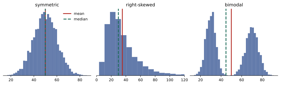
A distribution is summarized by its centre (mean, median), its spread (standard deviation, interquartile range, percentiles) and its shape (symmetric, skewed, multimodal). The right summary depends on the shape and on the decision being made. For power planning, the 95th percentile of server power often matters more than the mean; for skewed quantities such as costs or repair times, the median is more typical than the mean (Lesson 4).

import numpy as np
import pandas as pd

rng = np.random.default_rng(21)
watts = pd.DataFrame({
    "server": np.repeat(["cpu", "gpu"], [120, 40]),
    "watts": np.concatenate([rng.normal(420, 45, 120), rng.lognormal(np.log(2900), 0.18, 40)]).round(0),
})
print(watts.groupby("server")["watts"].describe(percentiles=[0.5, 0.95]).round(0).to_string())
print("Skewness:", watts.groupby("server")["watts"].skew().round(2).to_dict())

        count    mean    std     min     50%     95%     max
server
cpu     120.0   420.0   42.0   288.0   418.0   484.0   518.0
gpu      40.0  2831.0  484.0  2008.0  2688.0  3690.0  3807.0
Skewness: {'cpu': -0.2, 'gpu': 0.35}

Summarizing by group is essential when the data mixes populations. A single mean over all 160 servers, about 1,000 W, would describe neither kind of server: CPU servers draw about 420 W and GPU servers about 2,800 W. Skewness measures asymmetry: positive values mean a longer right tail, as with the GPU servers, whose occasional heavy workloads push the maximum well above the median.

Confidence intervals for a mean

The sample mean \(\bar{x}\) of \(n\) values estimates the population mean with standard error \(s/\sqrt{n}\). For small samples from roughly normal data, a 95% confidence interval uses the t distribution with \(n-1\) degrees of freedom:

The multiplier \(t_{0.975,\,n-1}\) is about 2.2 for 12 values and approaches 1.96 for large samples. The interpretation is subtle: if we repeated the study many times, 95% of intervals built this way would contain the true mean. In practice, a narrow interval means a precise estimate, and a wide one is a warning that more data is needed before drawing firm conclusions.

Comparing two groups: the t-test

Two sites report weekly PUE (power usage effectiveness, total facility power divided by IT power). Site B looks better. Is the difference real, and how big is it?

import numpy as np
from scipy import stats

rng = np.random.default_rng(4)
a = rng.normal(1.42, 0.06, 12)     # weekly PUE at site A
b = rng.normal(1.36, 0.05, 10)     # weekly PUE at site B

for name, x in [("A", a), ("B", b)]:
    lo, hi = stats.t.interval(0.95, len(x) - 1, loc=x.mean(), scale=stats.sem(x))
    print(f"Site {name}: mean {x.mean():.3f}, 95% CI {lo:.3f} to {hi:.3f}")

t, p = stats.ttest_ind(a, b, equal_var=False)       # Welch t-test
diff = a.mean() - b.mean()
pooled_sd = np.sqrt((a.var(ddof=1) + b.var(ddof=1)) / 2)
print(f"Difference {diff:.3f}, t = {t:.2f}, p = {p:.4f}, effect size d = {diff / pooled_sd:.2f}")

Site A: mean 1.419, 95% CI 1.379 to 1.459
Site B: mean 1.351, 95% CI 1.307 to 1.396
Difference 0.068, t = 2.54, p = 0.0198, effect size d = 1.09

The Welch t-test compares two means without assuming the groups have equal variances, which is the safer default. Here \(p \approx 0.02\): if the two sites really had the same mean PUE, a difference this large would arise by chance only about 2% of the time. The effect size, Cohen's \(d\), expresses the difference in standard deviations; \(d \approx 1.1\) is large.

Statistical significance is not the same as importance. With thousands of observations, a trivial difference of 0.001 in PUE would be "significant"; with a handful, an important difference might not be. Always report the size of the difference with its confidence interval, and judge it against what matters in practice. A PUE difference of 0.068 at a 20 MW site is worth about 1.4 MW of facility power.

Comparing proportions: A/B tests

Many AI products are evaluated with A/B tests: users are randomly assigned to the old version (A) or the new one (B), and an outcome such as clicks, purchases or problems resolved is compared. Random assignment is what makes the comparison fair: it balances every other factor, known or unknown, between the groups, so a difference can be attributed to the change.

import numpy as np
from scipy import stats

#                 resolved by bot, escalated
table = np.array([[1840, 1160],     # old help-desk assistant
                  [1972, 1028]])    # new assistant
rates = table[:, 0] / table.sum(axis=1)
print("Resolution rates:", np.round(rates, 3))

chi2, p, dof, expected = stats.chi2_contingency(table, correction=False)
print(f"chi-square = {chi2:.2f}, p = {p:.5f}")

n1, n2 = table.sum(axis=1)
diff = rates[1] - rates[0]
se = np.sqrt(rates[0] * (1 - rates[0]) / n1 + rates[1] * (1 - rates[1]) / n2)
print(f"Improvement {diff:.3f}, 95% CI {diff - 1.96 * se:.3f} to {diff + 1.96 * se:.3f}")

Resolution rates: [0.613 0.657]
chi-square = 12.53, p = 0.00040
Improvement 0.044, 95% CI 0.020 to 0.068

The new assistant resolved 65.7% of 3,000 requests against 61.3% for the old one. The chi-square test gives \(p = 0.0004\), so chance is a very unlikely explanation, and the 95% confidence interval says the true improvement is probably between 2.0 and 6.8 percentage points. The standard error of a difference in proportions is

Simpson's paradox

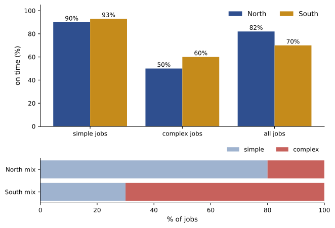
Aggregated data can point the opposite way from every one of its parts. Two maintenance teams handle simple and complex jobs. Which team is better at finishing on time?

import pandas as pd

jobs = pd.DataFrame({
    "team":   ["North"] * 2 + ["South"] * 2,
    "kind":   ["simple", "complex", "simple", "complex"],
    "jobs":   [80, 20, 30, 70],
    "on_time": [72, 10, 28, 42],
})
jobs["rate"] = jobs["on_time"] / jobs["jobs"]
print(jobs.pivot(index="kind", columns="team", values="rate").round(2).to_string())

overall = jobs.groupby("team")[["on_time", "jobs"]].sum()
print((overall["on_time"] / overall["jobs"]).round(2).to_string())

team     North  South
kind
complex    0.5   0.60
simple     0.9   0.93
team
North    0.82
South    0.70

South is better at both simple jobs (93% against 90%) and complex jobs (60% against 50%), yet North looks better overall (82% against 70%). The reason is the mix: 70% of South's jobs are complex, against 20% of North's, and complex jobs are late more often for everyone. Comparing the overall rates confounds team skill with job mix. This is Simpson's paradox, and it appears in medicine, admissions data, model evaluation and any comparison where groups differ in composition. The remedy is to compare like with like: stratify by the confounding variable, or adjust for it in a model, and above all think about what else differs between the groups.

Correlation and simple regression

Correlation measures how closely two variables follow a straight-line relationship, from −1 to +1 (Lesson 7). Regression goes further and fits a line \(y = a + bx\) by least squares, so that the slope \(b\) estimates how much \(y\) changes per unit of \(x\). The coefficient of determination \(R^{2}\) is the fraction of the variation in \(y\) that the line explains.

import numpy as np
from scipy import stats

rng = np.random.default_rng(12)
outside = rng.uniform(-15, 32, 60)                       # daily mean outdoor temperature, C
pue = 1.18 + 0.0062 * np.clip(outside, 5, None) + rng.normal(0, 0.012, 60)

fit = stats.linregress(outside, pue)
print(f"PUE = {fit.intercept:.3f} + {fit.slope:.4f} x temperature,  R^2 = {fit.rvalue**2:.2f}")

warm = outside >= 5
fit_warm = stats.linregress(outside[warm], pue[warm])
print(f"Warm days only: slope {fit_warm.slope:.4f} per C, R^2 = {fit_warm.rvalue**2:.2f}")
print("Mean PUE below 5 C:", round(pue[~warm].mean(), 3))

PUE = 1.229 + 0.0039 x temperature,  R^2 = 0.88
Warm days only: slope 0.0059 per C, R^2 = 0.95
Mean PUE below 5 C: 1.21

The fit over all days explains 88% of the variation, but the relationship is not really a straight line: below about 5 °C the site runs on free cooling and PUE stays flat, and above it PUE rises steeply. Fitting one line averages the two regimes and understates the warm-weather slope (0.0039 against 0.0059 per °C). Always plot the data and the residuals (the differences between the data and the fitted line) before trusting a fit; a curve, a kink or a fan-shaped spread in the residuals means the model is missing something.

Regression describes association, not causation. Outdoor temperature plausibly causes PUE changes through physics, but in other data, such as the relationship between the number of monitoring alerts and the number of outages, a third factor (a large, old, busy site) might drive both. Causal claims need either a controlled experiment, such as an A/B test, or careful reasoning about confounders.

A checklist for statistical claims

• What is the estimate, and what is its confidence interval?
• Is the effect large enough to matter in practice?
• How were the groups formed? Were they randomized? What else differs between them?
• How many comparisons were made before this one was reported (Lesson 4)?
• Do the data meet the method's assumptions (independence, roughly normal means, a straight-line relationship)? If not, use the bootstrap, a permutation test or a better model.
• Has the result been checked on new data?