An end-to-end project: from question to working model · AI-110 Lesson 12

This final lesson puts the whole course together in one project, the way it happens at work. A data centre operator wants to forecast tomorrow's cooling energy at each of its sites, so that it can buy electricity ahead of time, schedule chiller maintenance on mild days and spot sites whose cooling is drifting out of line. We will frame the problem, build the data set, set a baseline, train a model, analyze its errors, fix a problem the error analysis reveals, explain what the model has learned, and package it so that others can use it safely. The data is simulated so that every result can be reproduced, but every step and every mistake it guards against comes from real projects.

Step 1: frame the problem

Most failed AI projects fail before any code is written, because the question was vague or the success measure did not match the business need. Before touching data, write down:

The decision the model supports: buying day-ahead electricity and planning maintenance.
The prediction: total cooling energy (MWh) for each site for the next day.
What is known at prediction time: the site, the forecast outdoor temperature, the expected IT load and the day of the week. Anything measured during the day being predicted is off limits (Lesson 6).
The success measure: mean absolute error (MAE) in MWh, because errors cost money roughly in proportion to their size. Also the bias (average signed error), because consistent under-forecasting leads to buying too little power.
The baseline to beat, and what accuracy would be good enough to be useful.

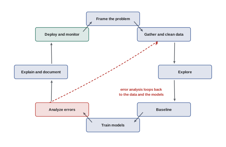
A machine learning project is a loop, not a straight line.

Step 2: build the data set and a baseline

Two years of daily records for three sites give 2,190 rows. Because the model will forecast the future, the data is split by time: everything before May 1, 2026 trains the model, and the six months after it test the model, just as it would be used. A random split would let the model train on days surrounding each test day and look better than it really is.

The baseline is deliberately simple: tomorrow will look like the same day last week at the same site. Any model that cannot beat this is not worth deploying.

Building the data set, splitting by date and scoring a "same day last week" baseline.

import numpy as np
import pandas as pd

rng = np.random.default_rng(12)
days = pd.date_range("2024-11-01", "2026-10-31", freq="D")
frames = []
for site, base_t, it in [("YYZ-1", 9, 30.0), ("ORD-2", 11, 42.0), ("PHX-1", 24, 18.0)]:
    doy = days.dayofyear.to_numpy()
    temp = base_t + 13 * np.sin(2 * np.pi * (doy - 110) / 365) + rng.normal(0, 3.5, len(days))
    it_mw = it * (1 + 0.25 * np.arange(len(days)) / len(days)) + rng.normal(0, 0.6, len(days))
    cooling = 24 * it_mw * (0.07 + 0.0055 * np.clip(temp - 8, 0, None)) + rng.normal(0, 4, len(days))
    frames.append(pd.DataFrame({"date": days, "site": site, "temp_c": temp.round(1),
                                "it_mw": it_mw.round(2), "cooling_mwh": cooling.round(1)}))
df = pd.concat(frames, ignore_index=True)
df["weekday"] = df["date"].dt.dayofweek
print(df.shape, "|", df["date"].min().date(), "to", df["date"].max().date())
print(df.groupby("site")["cooling_mwh"].agg(["mean", "min", "max"]).round(1).to_string())

cutoff = pd.Timestamp("2026-05-01")
train, test = df[df["date"] < cutoff], df[df["date"] >= cutoff]
print(f"Train {len(train)} rows (before {cutoff.date()}), test {len(test)} rows")

# Baseline: tomorrow will look like the same site a week ago
df["last_week"] = df.groupby("site")["cooling_mwh"].shift(7)
base = df.loc[test.index].dropna(subset=["last_week"])
mae = (base["cooling_mwh"] - base["last_week"]).abs().mean()
print(f"Baseline (same day last week) MAE: {mae:.1f} MWh")

Output

(2190, 6) | 2024-11-01 to 2026-10-31
        mean   min    max
site
ORD-2  116.0  60.3  237.2
PHX-1   77.8  25.7  144.5
YYZ-1   78.9  39.0  170.8
Train 1638 rows (before 2026-05-01), test 552 rows
Baseline (same day last week) MAE: 20.3 MWh

The baseline's MAE is about 20 MWh, against typical daily values of 80 to 120 MWh. That sets the bar.

Step 3: train a model

A gradient-boosted tree model (Lesson 9) is a strong default for tabular data. The site is one-hot encoded inside a pipeline, and the numeric features pass through unchanged, since tree models do not need scaling.

A gradient-boosted model of daily cooling energy, evaluated on the six held-out months, with errors broken down by site.

import numpy as np
import pandas as pd

rng = np.random.default_rng(12)
days = pd.date_range("2024-11-01", "2026-10-31", freq="D")
frames = []
for site, base_t, it in [("YYZ-1", 9, 30.0), ("ORD-2", 11, 42.0), ("PHX-1", 24, 18.0)]:
    doy = days.dayofyear.to_numpy()
    temp = base_t + 13 * np.sin(2 * np.pi * (doy - 110) / 365) + rng.normal(0, 3.5, len(days))
    it_mw = it * (1 + 0.25 * np.arange(len(days)) / len(days)) + rng.normal(0, 0.6, len(days))
    cooling = 24 * it_mw * (0.07 + 0.0055 * np.clip(temp - 8, 0, None)) + rng.normal(0, 4, len(days))
    frames.append(pd.DataFrame({"date": days, "site": site, "temp_c": temp.round(1),
                                "it_mw": it_mw.round(2), "cooling_mwh": cooling.round(1)}))
df = pd.concat(frames, ignore_index=True)
df["weekday"] = df["date"].dt.dayofweek
from sklearn.compose import ColumnTransformer
from sklearn.ensemble import HistGradientBoostingRegressor
from sklearn.pipeline import make_pipeline
from sklearn.preprocessing import OneHotEncoder

features = ["site", "temp_c", "it_mw", "weekday"]
cutoff = pd.Timestamp("2026-05-01")
train, test = df[df["date"] < cutoff], df[df["date"] >= cutoff]

prep = ColumnTransformer([("site", OneHotEncoder(), ["site"])], remainder="passthrough")
model = make_pipeline(prep, HistGradientBoostingRegressor(max_iter=300, learning_rate=0.05, random_state=0))
model.fit(train[features], train["cooling_mwh"])

pred = model.predict(test[features])
err = test["cooling_mwh"] - pred
mape = (err.abs() / test["cooling_mwh"]).mean()
print(f"Model MAE: {err.abs().mean():.1f} MWh | MAPE: {mape:.1%}")
test = test.assign(error=err)
print(test.groupby("site")["error"].agg(mae=lambda e: e.abs().mean(), bias="mean").round(1).to_string())

Output

Model MAE: 7.0 MWh | MAPE: 5.3%
        mae  bias
site
ORD-2  11.4  11.0
PHX-1   5.4   3.3
YYZ-1   4.3   2.3

The overall MAE of 7.0 MWh is about a third of the baseline's, a large improvement. A less careful project would stop here. But the breakdown by site tells a different story: at ORD-2 the model under-forecasts by 11 MWh on average, every day. A consistent bias like this is a sign that something systematic is wrong, and it would cause the operator to buy too little electricity at its largest site.

Step 4: analyze the errors

Error analysis means slicing the errors by every variable that might matter, site, season, load level, day of week, and asking why the worst slices are bad. Here the cause is growth. ORD-2's IT load grew steadily over the two years, and in the test period it ran higher than at any time in the training data. Tree-based models cannot extrapolate: for inputs beyond the training range they predict roughly the value at the edge of that range. So the model treats a 53 MW day as if it were a 51 MW day, and under-forecasts.

The fix comes from understanding the physics rather than from a more complex model. Cooling energy scales roughly in proportion to IT energy, so instead of predicting cooling energy directly, the model predicts the ratio of cooling energy to IT energy, which depends mainly on weather and stays in the same range as the load grows. The forecast is then the predicted ratio multiplied by the expected IT energy.

Predicting cooling energy per unit of IT energy removes the extrapolation problem.

import numpy as np
import pandas as pd

rng = np.random.default_rng(12)
days = pd.date_range("2024-11-01", "2026-10-31", freq="D")
frames = []
for site, base_t, it in [("YYZ-1", 9, 30.0), ("ORD-2", 11, 42.0), ("PHX-1", 24, 18.0)]:
    doy = days.dayofyear.to_numpy()
    temp = base_t + 13 * np.sin(2 * np.pi * (doy - 110) / 365) + rng.normal(0, 3.5, len(days))
    it_mw = it * (1 + 0.25 * np.arange(len(days)) / len(days)) + rng.normal(0, 0.6, len(days))
    cooling = 24 * it_mw * (0.07 + 0.0055 * np.clip(temp - 8, 0, None)) + rng.normal(0, 4, len(days))
    frames.append(pd.DataFrame({"date": days, "site": site, "temp_c": temp.round(1),
                                "it_mw": it_mw.round(2), "cooling_mwh": cooling.round(1)}))
df = pd.concat(frames, ignore_index=True)
df["weekday"] = df["date"].dt.dayofweek
from sklearn.compose import ColumnTransformer
from sklearn.ensemble import HistGradientBoostingRegressor
from sklearn.pipeline import make_pipeline
from sklearn.preprocessing import OneHotEncoder

features = ["site", "temp_c", "weekday"]
cutoff = pd.Timestamp("2026-05-01")
train, test = df[df["date"] < cutoff], df[df["date"] >= cutoff]
o_tr, o_te = train[train.site == "ORD-2"].it_mw, test[test.site == "ORD-2"].it_mw
print(f"ORD-2 IT load: train {o_tr.min():.1f}-{o_tr.max():.1f} MW, test {o_te.min():.1f}-{o_te.max():.1f} MW")

# Predict cooling energy per MWh of IT energy, then scale back up
ratio = train["cooling_mwh"] / (24 * train["it_mw"])
prep = ColumnTransformer([("site", OneHotEncoder(), ["site"])], remainder="passthrough")
model = make_pipeline(prep, HistGradientBoostingRegressor(max_iter=300, learning_rate=0.05, random_state=0))
model.fit(train[features], ratio)

pred = model.predict(test[features]) * 24 * test["it_mw"]
test = test.assign(error=test["cooling_mwh"] - pred)
print(f"Model MAE: {test.error.abs().mean():.1f} MWh")
print(test.groupby("site")["error"].agg(mae=lambda e: e.abs().mean(), bias="mean").round(1).to_string())

Output

ORD-2 IT load: train 41.3-51.0 MW, test 48.6-53.5 MW
Model MAE: 3.8 MWh
       mae  bias
site
ORD-2  4.1   0.4
PHX-1  4.0   0.5
YYZ-1  3.3  -0.0

The overall MAE falls from 7.0 to 3.8 MWh, and the bias at ORD-2 falls from 11 MWh to almost nothing. Reframing the target using domain knowledge did more than any amount of hyperparameter tuning could have. This is typical: the biggest gains in applied machine learning usually come from better framing, better data and better features, not from more elaborate algorithms.

Worked problem

What the improvement is worth

The operator buys day-ahead power for cooling. Each MWh of forecast error costs on average $25 in imbalance charges and missed savings. Across the three sites, what is the annual cost of forecast error with the baseline, the first model and the improved model?

Show solution

Daily site-forecasts per year: $3 \times 365 = 1{,}095$.
Baseline: $1{,}095 \times 20.3 \times 25 = \$555{,}700$.
First model: $1{,}095 \times 7.0 \times 25 = \$191{,}600$.
Improved model: $1{,}095 \times 3.8 \times 25 = \$104{,}000$.

Answer: About $556,000, $192,000 and $104,000 a year. The first model saves about $364,000 over the baseline, and the error analysis saves a further $88,000, while also removing the systematic under-buying at the largest site. Translating metrics into money, as in Lesson 9, is how projects earn support.

Step 5: explain the model

Users trust, and correctly use, models they understand. Permutation importance measures how much a model relies on each feature: shuffle one feature's values in the test data, breaking its link to the target, and see how much the error grows. Unlike the built-in importances of tree models, it is measured on held-out data and works with any model.

Permutation importance of each feature for the cooling-ratio model.

import numpy as np
import pandas as pd

rng = np.random.default_rng(12)
days = pd.date_range("2024-11-01", "2026-10-31", freq="D")
frames = []
for site, base_t, it in [("YYZ-1", 9, 30.0), ("ORD-2", 11, 42.0), ("PHX-1", 24, 18.0)]:
    doy = days.dayofyear.to_numpy()
    temp = base_t + 13 * np.sin(2 * np.pi * (doy - 110) / 365) + rng.normal(0, 3.5, len(days))
    it_mw = it * (1 + 0.25 * np.arange(len(days)) / len(days)) + rng.normal(0, 0.6, len(days))
    cooling = 24 * it_mw * (0.07 + 0.0055 * np.clip(temp - 8, 0, None)) + rng.normal(0, 4, len(days))
    frames.append(pd.DataFrame({"date": days, "site": site, "temp_c": temp.round(1),
                                "it_mw": it_mw.round(2), "cooling_mwh": cooling.round(1)}))
df = pd.concat(frames, ignore_index=True)
df["weekday"] = df["date"].dt.dayofweek
from sklearn.ensemble import HistGradientBoostingRegressor
from sklearn.inspection import permutation_importance

df["site_code"] = df["site"].map({"YYZ-1": 0, "ORD-2": 1, "PHX-1": 2})
features = ["site_code", "temp_c", "weekday"]
cutoff = pd.Timestamp("2026-05-01")
train, test = df[df["date"] < cutoff], df[df["date"] >= cutoff]
y_train = train["cooling_mwh"] / (24 * train["it_mw"])
y_test = test["cooling_mwh"] / (24 * test["it_mw"])

model = HistGradientBoostingRegressor(max_iter=300, learning_rate=0.05, random_state=0,
                                      categorical_features=[0]).fit(train[features], y_train)
result = permutation_importance(model, test[features], y_test, n_repeats=10, random_state=0,
                                scoring="neg_mean_absolute_error")
for name, imp in sorted(zip(features, result.importances_mean), key=lambda p: -p[1]):
    print(f"{name:>10}: MAE rises by {imp:.4f} when shuffled")

Output

    temp_c: MAE rises by 0.0481 when shuffled
 site_code: MAE rises by 0.0001 when shuffled
   weekday: MAE rises by -0.0001 when shuffled

Shuffling temperature makes the error much worse, while shuffling the site or the weekday changes almost nothing: the ratio of cooling to IT energy depends on the weather, and once that is known the sites behave alike. That matches engineering intuition, which is reassuring. When importances contradict intuition, investigate: either the model has found something real and surprising, or, more often, it has found a leak or an artifact in the data. Tools such as partial dependence plots and SHAP values go further, showing how each feature moves individual predictions.

Step 6: package and deploy

A model in a notebook helps nobody else. Deployment means making predictions available where decisions are made: a scheduled job that writes tomorrow's forecasts to a database, or a small web service that other systems call. Whatever the form, the package should include:

The trained model, saved to a file (joblib for scikit-learn models), with a version number.
The exact preprocessing, ideally inside the saved pipeline so that it cannot drift from what was used in training.
Input validation that rejects or flags inputs the model was not trained for.
A model card: a short document stating what the model predicts, the data and period it was trained on, its measured performance, its valid input ranges, its known limitations and who owns it.

Saving the model and a model card, loading it as a service would, and wrapping it in a forecast function that validates its inputs.

import numpy as np
import pandas as pd

rng = np.random.default_rng(12)
days = pd.date_range("2024-11-01", "2026-10-31", freq="D")
frames = []
for site, base_t, it in [("YYZ-1", 9, 30.0), ("ORD-2", 11, 42.0), ("PHX-1", 24, 18.0)]:
    doy = days.dayofyear.to_numpy()
    temp = base_t + 13 * np.sin(2 * np.pi * (doy - 110) / 365) + rng.normal(0, 3.5, len(days))
    it_mw = it * (1 + 0.25 * np.arange(len(days)) / len(days)) + rng.normal(0, 0.6, len(days))
    cooling = 24 * it_mw * (0.07 + 0.0055 * np.clip(temp - 8, 0, None)) + rng.normal(0, 4, len(days))
    frames.append(pd.DataFrame({"date": days, "site": site, "temp_c": temp.round(1),
                                "it_mw": it_mw.round(2), "cooling_mwh": cooling.round(1)}))
df = pd.concat(frames, ignore_index=True)
df["weekday"] = df["date"].dt.dayofweek
import json
import joblib
from sklearn.ensemble import HistGradientBoostingRegressor

SITES = {"YYZ-1": 0, "ORD-2": 1, "PHX-1": 2}
df["site_code"] = df["site"].map(SITES)
features = ["site_code", "temp_c", "weekday"]
train = df[df["date"] < "2026-05-01"]
model = HistGradientBoostingRegressor(max_iter=300, learning_rate=0.05, random_state=0,
                                      categorical_features=[0])
model.fit(train[features], train["cooling_mwh"] / (24 * train["it_mw"]))
joblib.dump(model, "cooling_model.joblib")

card = {"name": "daily-cooling-energy", "version": "1.0.0", "trained_through": "2026-04-30",
        "target": "cooling MWh per MWh of IT energy", "test_mae_mwh": 3.8,
        "valid_sites": sorted(SITES), "valid_temp_c": [float(train.temp_c.min()), float(train.temp_c.max())]}
with open("model_card.json", "w", encoding="utf-8") as f:
    json.dump(card, f, indent=2)

loaded = joblib.load("cooling_model.joblib")      # as a separate service would

def forecast(site, temp_c, it_mw, weekday):
    if site not in SITES:
        raise ValueError(f"unknown site {site}")
    lo, hi = card["valid_temp_c"]
    note = "" if lo <= temp_c <= hi else "  (warning: temperature outside training range)"
    X = pd.DataFrame([[SITES[site], temp_c, weekday]], columns=features)
    return round(float(loaded.predict(X)[0]) * 24 * it_mw, 1), note

print(forecast("YYZ-1", 27.0, 38.0, 2))
print(forecast("PHX-1", 49.0, 23.0, 5))
try:
    forecast("LAX-9", 20.0, 10.0, 1)
except ValueError as err:
    print("Rejected:", err)

Output

(161.4, '')
(132.4, '  (warning: temperature outside training range)')
Rejected: unknown site LAX-9

The forecast function refuses an unknown site outright and flags a temperature of 49 °C, hotter than anything in the training data, where the prediction is an extrapolation and should not be trusted blindly. In production, flagged forecasts would be logged and shown to a person.

Step 7: monitor and maintain

A deployed model starts to age immediately. The world it learned from changes: new cooling equipment is installed, IT load grows, a site changes its operating temperature set points, the climate shifts. Monitoring watches for this:

Prediction quality: once the actual values arrive, track MAE and bias over time and by site, with alerts when they degrade.
Data drift: compare the distributions of incoming features with those in the training data; values outside the training range are an early warning.
Data quality: apply the validation checks of Lesson 6 to every batch of inputs.
Retraining: retrain on recent data on a schedule or when monitoring shows degradation, and evaluate each new version against the old one on the same recent data before switching.

The operational discipline of versioning, testing, deploying and monitoring models is called MLOps, and it is the subject of AI-420.

Responsible practice

Even a model as harmless-seeming as an energy forecast raises questions of responsibility: who is accountable if a bad forecast leads to an expensive purchase, how will users know when not to trust it, and is anyone affected who was not consulted? Models that make decisions about people, such as hiring, lending, access to services or performance evaluation, raise much more serious questions of fairness, privacy and transparency, and are increasingly regulated.

In Canada, federal institutions using automated decision systems must follow the Treasury Board Directive on Automated Decision-Making, including algorithmic impact assessments, and privacy laws apply to personal data used in training. Organizations should document their models, test them for bias across groups, and keep a person accountable for decisions.

Where to go from here

This course has given you the working toolkit of a data and AI practitioner: Python and its data libraries, data cleaning, visualization, statistics, simulation, databases, machine learning and reproducible projects. The next steps in the program build on it: the mathematics behind machine learning (AI-210), data engineering and visualization at scale (AI-220), optimization, probabilistic models and reinforcement learning, deep learning for language and vision, and machine learning systems in production (AI-420). The best way to consolidate what you have learned is to carry a project of your own from question to working model, as this lesson did, using data from a field you care about.

Common mistakes

MistakeStarting with an algorithm instead of a decision and a success measure.
InsteadFrame the decision, the prediction, the available inputs and the metric first.
MistakeSkipping the baseline.
InsteadScore a simple baseline so you know whether the model adds value.
MistakeStopping at a good overall metric.
InsteadBreak errors down by segment and look for bias.
MistakeExpecting tree models to extrapolate beyond the training range.
InsteadReframe the target or features so that new data stays within the learned range, and flag inputs outside it.
MistakeDeploying a model without validation, documentation or monitoring.
InsteadShip input checks, a model card and monitoring with every model.

Summary and key terms

Frame the decision, prediction, inputs available at prediction time and success measure first.
Split by time for forecasting and beat a simple baseline.
Error analysis by segment reveals problems that overall metrics hide.
Tree models cannot extrapolate; reframing the target with domain knowledge fixed the bias.
Permutation importance explains which features the model relies on.
Deploy with a saved pipeline, input validation and a model card.
Monitor quality, drift and data, retrain deliberately, and keep people accountable.

Problem framing: Defining the decision, prediction, inputs and success measure of a project.
Baseline: A simple reference prediction a model must beat.
Bias (of a forecast): The average signed error; consistent over- or under-prediction.
Error analysis: Breaking down errors by segment to find their causes.
Extrapolation: Predicting for inputs outside the range of the training data.
Permutation importance: The increase in error when a feature's values are shuffled.
Model card: A short document describing a model's purpose, data, performance and limits.
Deployment: Making a model's predictions available where decisions are made.
Data drift: A change in the distribution of incoming data compared with training data.
MLOps: Practices for versioning, deploying and monitoring models.

Practice problems

Work each problem on paper first, then reveal the answer to check.

Name four things to write down before starting a modelling project.
Show answer
The decision, the prediction, the inputs available at prediction time and the success measure (and the baseline).
Why split forecasting data by time?
Show answer
To mimic real use and avoid training on days around the test days.
What baseline did the project use?
Show answer
The same site's value on the same day of the previous week.
A site's average error is +11 MWh. What does that indicate?
Show answer
A systematic bias: the model consistently under-forecasts there.
Why did the tree model under-forecast ORD-2?
Show answer
Its IT load exceeded the training range, and trees cannot extrapolate.
How was the problem fixed?
Show answer
By predicting cooling energy per unit of IT energy and scaling back up.
Error falls from 7.0 to 3.8 MWh on 1,095 forecasts a year at $25/MWh. Annual saving?
Show answer
About $87,600.
How is permutation importance measured?
Show answer
By shuffling one feature in held-out data and measuring how much the error grows.
What belongs in a model card?
Show answer
Purpose, training data and period, performance, valid input ranges, limitations and owner.
Name two things to monitor after deployment.
Show answer
Prediction error and bias over time, and drift in input data (also data quality).