Arrays and vectorized computation with NumPy

Machine learning is arithmetic on large blocks of numbers. An image is a grid of pixel values; a batch of images is a stack of grids. A data set of a million sensor readings with twenty features each is a table of twenty million numbers. A neural network layer is a matrix of weights multiplied by a matrix of inputs. Python lists can hold numbers, but they are slow to compute with and awkward for anything beyond one dimension.

NumPy (Numerical Python) solves this with one central object, the n-dimensional array, and a large library of fast operations on it. Almost every scientific and AI library in Python is built on NumPy or copies its design: pandas stores its columns in NumPy arrays, scikit-learn takes NumPy arrays as input, and PyTorch tensors and JAX arrays behave almost exactly like NumPy arrays, with the addition of GPUs and automatic differentiation. Learn NumPy well and you have learned the grammar of numerical Python.

The ndarray

A NumPy array is a block of numbers that all share one data type, laid out contiguously in memory, with a shape that says how many elements lie along each axis. Three attributes describe it:

• shape: a tuple of sizes along each axis, such as (3, 4) for 3 rows and 4 columns.
• ndim: the number of axes (dimensions). A vector has 1, a table 2, a colour image 3 (height, width, colour channel), and a batch of colour images 4.
• dtype: the data type of every element, such as float64 (64-bit floating point, the default), float32, int64 or bool.

Because every element has the same type and the data is packed together, NumPy can hand the whole block to compiled code that loops over it at machine speed. That is the source of its performance.

import numpy as np

# Power in kW: 3 racks (rows) x 4 hours (columns)
power = np.array([[11.2, 12.0, 11.8, 12.4],
                  [ 8.9,  9.3,  9.1,  9.6],
                  [15.1, 15.8, 16.2, 15.5]])
print(power.shape, power.ndim, power.size, power.dtype)
print(power.sum())            # every value
print(power.sum(axis=1))      # per rack: add across the hours
print(power.mean(axis=0).round(2))   # per hour: average across the racks
print(power[2, 1], power[:, 0], power[1])

(3, 4) 2 12 float64
146.9
[47.4 36.9 62.6]
[11.73 12.37 12.37 12.5 ]
15.8 [11.2  8.9 15.1] [8.9 9.3 9.1 9.6]

Axes

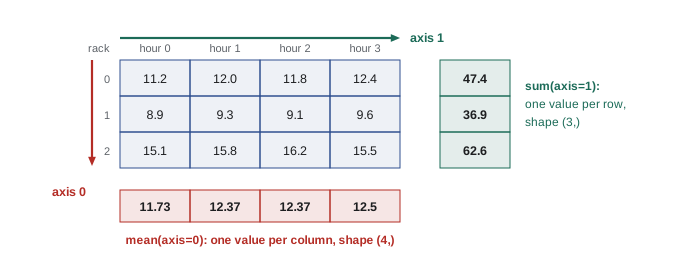
The axis argument is the most important idea in this chapter, and the most common source of confusion. An aggregation such as sum, mean or max along an axis collapses that axis. For a two-dimensional array:

• axis=0 runs down the rows, so the result has one value per column. power.mean(axis=0) averages the three racks for each hour.
• axis=1 runs across the columns, so the result has one value per row. power.sum(axis=1) adds up the four hours for each rack.
• No axis aggregates every element into one number.

A reliable way to remember: the axis you name is the one that disappears. A (3, 4) array summed over axis=1 becomes shape (3,); summed over axis=0 it becomes shape (4,). In a batch of images with shape (batch, height, width, channels), averaging over axes (1, 2) gives the mean colour of each image, shape (batch, channels).

Indexing and slicing

Arrays are indexed with one index per axis, separated by commas: power[2, 1] is row 2, column 1 (counting from zero), which is 15.8. Slices work along each axis as they do for lists: power[:, 0] takes every row in column 0, and power[1] takes the whole of row 1. Slices can also have steps: x[::2] takes every second element, and x[::-1] reverses an array.

Creating arrays

Besides converting lists with np.array, NumPy has functions that create arrays directly: np.zeros((3, 4)) and np.ones(5) for filled arrays, np.arange(0, 10, 2) for evenly stepped integers, np.linspace(0, 1, 11) for a given number of evenly spaced points (including both ends), and the random generator described later. The method .reshape changes the shape without changing the data, as long as the number of elements stays the same: np.arange(12).reshape(3, 4).

Vectorization

Writing an operation on whole arrays, instead of looping over elements in Python, is called vectorization. An expression such as x * x squares every element; np.sqrt(x), np.exp(x) and np.log(x) apply a function to every element; and comparisons such as x > 25 produce an array of True and False values. These element-wise functions are called universal functions (ufuncs). The loop still happens, but inside NumPy's compiled code rather than in the Python interpreter.

The speed difference is dramatic:

import time
import numpy as np

x = np.random.default_rng(0).random(1_000_000)

t0 = time.perf_counter()
total = 0.0
for v in x:                    # one element at a time, in Python
    total += v * v
t1 = time.perf_counter()
fast = np.sum(x * x)           # the whole array at once, in compiled code
t2 = time.perf_counter()

print(f"loop:  {t1 - t0:.3f} s")
print(f"numpy: {t2 - t1:.4f} s")
print(np.isclose(total, fast))

loop:  0.128 s
numpy: 0.0045 s
True

The exact times depend on your computer, but the vectorized version is typically 20 to 100 times faster, and the gap grows with more complex operations. The two results agree to within rounding (they add in a slightly different order, which is why the comparison uses np.isclose). In AI work this is not a minor optimization: it is the difference between a data-preparation step taking a minute or an hour. The same principle, applied on GPUs, is what makes deep learning feasible.

Broadcasting

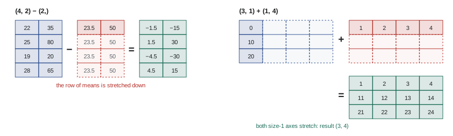
Element-wise operations need arrays of compatible shapes. Broadcasting is NumPy's set of rules for combining arrays of different shapes without copying data. The rules compare shapes from the rightmost axis leftwards; two sizes are compatible if they are equal or if one of them is 1, and a missing axis counts as size 1. The size-1 axis is then stretched (conceptually) to match the other.

The simplest case is an array and a single number: X * 2 multiplies every element. A more useful case is combining a table with one value per column. A (4, 2) table minus a (2,) vector of column means subtracts each column's mean from every row in that column. This is exactly how features are standardized before training many machine learning models.

import numpy as np

# Features for 4 servers: inlet temperature (°C) and CPU load (%)
X = np.array([[22.0, 35.0],
              [25.0, 80.0],
              [19.0, 20.0],
              [28.0, 65.0]])
mean = X.mean(axis=0)          # shape (2,)
std = X.std(axis=0)            # shape (2,)
Z = (X - mean) / std           # (4, 2) minus (2,): broadcast down the rows
print(mean, std.round(3))
print(Z.round(3))
print(Z.mean(axis=0).round(6), Z.std(axis=0))

[23.5 50. ] [ 3.354 23.717]
[[-0.447 -0.632]
 [ 0.447  1.265]
 [-1.342 -1.265]
 [ 1.342  0.632]]
[0. 0.] [1. 1.]

After standardizing, each column has mean 0 and standard deviation 1, so temperature (a few degrees of spread) and load (tens of percent) are on a comparable scale. Gradient-based training, which you met in AI-101, converges far better on standardized features.

Boolean masks and selection

A comparison such as temps > 27 returns a Boolean array of the same shape. That array can be used as an index to select only the elements where it is True, which is called boolean masking. It replaces loops containing if statements, and it is the basis of filtering rows in pandas.

import numpy as np

temps = np.array([22.4, 23.1, 27.9, 24.0, 28.6, 21.8, 26.2])
racks = np.array(["A1", "A2", "A3", "B1", "B2", "B3", "C1"])
hot = temps > 27
print(hot)
print(racks[hot], temps[hot])
print(np.count_nonzero(temps > 25), "racks above 25 °C")
print(np.where(temps > 27, 27.0, temps))
order = np.argsort(temps)[::-1]
print(racks[order[:3]])

[False False  True False  True False False]
['A3' 'B2'] [27.9 28.6]
3 racks above 25 °C
[22.4 23.1 27.  24.  27.  21.8 26.2]
['B2' 'A3' 'C1']

A mask from one array can select from another array of the same length, as racks[hot] does, which keeps related data aligned. Masks combine with & (and), | (or) and ~ (not), with each comparison in parentheses: (temps > 22) & (temps < 25). np.where(condition, a, b) picks from a where the condition is true and from b elsewhere; here it caps the temperatures at 27. np.argsort returns the indices that would sort the array, which lets you sort one array by the values of another.

Linear algebra

Machine learning models are, at their core, sequences of matrix operations, and NumPy provides them. The @ operator performs matrix multiplication (np.matmul): for an (n, d) matrix X and a vector w of length d, X @ w gives the n predictions of a linear model in one operation. Note that X * w is something different: element-wise multiplication with broadcasting. The np.linalg module solves linear systems, computes inverses, determinants, eigenvalues and decompositions, and fits least-squares models.

import numpy as np

# Server power model: P = idle + per_core * busy_cores + per_gb * memory_gb
X = np.array([[1, 10, 64],
              [1, 24, 128],
              [1, 40, 256],
              [1, 56, 256],
              [1, 64, 512]], dtype=float)     # columns: constant, busy cores, memory GB
w_true = np.array([120.0, 4.5, 0.25])          # W, W per core, W per GB
rng = np.random.default_rng(42)
P = X @ w_true + rng.normal(0, 3, size=5)      # measured power with noise
print(P.round(1))
w, *_ = np.linalg.lstsq(X, P, rcond=None)      # least-squares fit
print(w.round(2))
print((X @ w).round(1))

[181.9 256.9 366.3 438.8 530.1]
[119.83   4.72   0.21]
[180.7 260.4 363.2 438.8 531. ]

The program simulates measurements from a known model (120 W idle, 4.5 W per busy core, 0.25 W per GB of memory) plus random noise, then recovers the coefficients with least squares. The fit finds about 120 W, 4.7 W per core and 0.21 W per GB: close to the truth, but not exact, because five noisy measurements cannot pin down three parameters perfectly. With more data the estimates would tighten. The column of ones in X lets the model learn the constant (intercept) term, a standard trick.

Random numbers

Simulation, data splitting, weight initialization and data augmentation all need random numbers. Modern NumPy code creates a generator with rng = np.random.default_rng(seed) and calls methods on it: rng.random(5) for uniform values between 0 and 1, rng.normal(mean, sd, size) for normally distributed values, rng.integers(low, high, size), rng.choice and rng.permutation. The seed makes the sequence repeatable: the same seed always gives the same numbers, which is essential for reproducible experiments (Lesson 11). Lesson 4 puts random generators to work in simulations and the bootstrap. Older tutorials use functions such as np.random.rand directly; the generator style is preferred in new code because each part of a program can have its own independent, seeded stream.

Views and copies

For speed, NumPy avoids copying data when it can. Slicing an array returns a view: a new array object that looks at the same memory. Changing the view changes the original. Reshaping and transposing usually return views too. Boolean masks and integer-list indexing, by contrast, always return copies.

import numpy as np

a = np.arange(6)
view = a[1:4]          # slicing gives a view: no data is copied
view[0] = 99
print(a)
b = np.arange(6)
copy = b[1:4].copy()   # an independent copy
copy[0] = 99
print(b)
c = a.reshape(2, 3)    # also a view of the same data
print(c.shape, np.shares_memory(a, c))

[ 0 99  2  3  4  5]
[0 1 2 3 4 5]
(2, 3) True

Views make NumPy fast and memory-efficient, which matters when arrays hold gigabytes, but they cause subtle bugs when a function modifies what it thinks is its own data. When you need an independent array, call .copy() explicitly.

Data types and memory

Every element of an array has the same dtype, and the dtype decides both precision and memory. A float64 element uses 8 bytes, float32 uses 4 and float16 uses 2. An array of 100 million float64 values occupies 800 MB; the same data as float32 needs 400 MB. Deep learning usually trains in float32, bfloat16 or float16 to halve or quarter memory and speed up computation. The .astype method converts between types, and .nbytes reports an array's size in bytes. Integer types can overflow silently: an int8 holds only −128 to 127, so 127 + 1 wraps around to −128. Choose types deliberately when memory or exactness matters.