
AI-110 · Lesson 7 of 12 · 30 min
Plotting and exploratory analysis
Before training any model, an experienced practitioner looks at the data. Not at summary numbers alone, but at pictures: how each variable is distributed, how variables relate to each other, where the gaps, spikes and oddities are. This stage is called exploratory data analysis (EDA). It catches errors that would otherwise poison a model, suggests which features matter, and often answers the original question without any machine learning at all.
Plots are also how results are communicated. A clear chart in a report or presentation persuades in a way a table of numbers rarely does, and a misleading chart can do real damage. This chapter introduces Matplotlib, the foundational plotting library in Python, then walks through the EDA process with examples. Every chart in this chapter was produced by the code shown with it.
Matplotlib basics: figures and axes
Matplotlib can draw almost any kind of chart, and most other Python plotting libraries (including pandas' .plot method and seaborn) are built on it. Its design has two key objects:
- A Figure is the whole image or window. It can contain one or more plots.
- An Axes (note the singular is still "Axes") is one plot within the figure: the area with an x-axis, a y-axis, the data and its labels.
The recommended style creates both at once with fig, ax = plt.subplots() and then calls methods on ax to draw and label: ax.plot for lines, ax.scatter for points, ax.bar for bars, ax.hist for histograms, and ax.set_xlabel, ax.set_ylabel and ax.set_title for labels. Matplotlib also has an older, shorter style (plt.plot, plt.xlabel and so on) that acts on whichever plot is current. It is fine for a quick look, but the explicit ax style is clearer as soon as a figure has more than one plot.
import numpy as np
import matplotlib.pyplot as plt

hours = np.arange(24)
it_load = 800 + 120 * np.sin((hours - 9) / 24 * 2 * np.pi)     # kW
facility = it_load * (1.25 + 0.10 * np.sin((hours - 10) / 24 * 2 * np.pi))

fig, ax = plt.subplots(figsize=(7, 3.5))
ax.plot(hours, facility, label="Facility total", color="tab:red")
ax.plot(hours, it_load, label="IT equipment", color="tab:blue")
ax.set_xlabel("Hour of day")
ax.set_ylabel("Power (kW)")
ax.set_title("One day of power use")
ax.set_xticks(range(0, 24, 3))
ax.grid(alpha=0.3)
ax.legend()
fig.tight_layout()
fig.savefig("daily_load.png", dpi=150)
print(f"PUE ranges from {(facility / it_load).min():.2f} to {(facility / it_load).max():.2f}")PUE ranges from 1.15 to 1.35
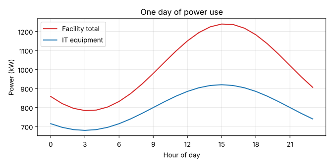
A few habits make every chart better, and the example shows them all:
- Label both axes, with units. "Power (kW)" is useful; "y" is not.
- Add a legend whenever there is more than one series, or label the lines directly.
- Keep gridlines light (alpha=0.3) so they help reading values without dominating.
- Call fig.tight_layout() so labels are not cut off, and save with fig.savefig. PNG at 150 dpi or more suits documents and slides; SVG or PDF keep lines sharp at any size.
In a notebook, the figure appears below the cell automatically. In a script, plt.show() opens a window, or the figure is saved to a file as here.
Choosing the right chart
Each common chart type answers a different kind of question:
| Question | Chart | Matplotlib |
|---|---|---|
| How does a value change over time or along an ordered variable? | Line chart | ax.plot |
| How are the values of one variable distributed? | Histogram (or box plot) | ax.hist, ax.boxplot |
| How do two numeric variables relate? | Scatter plot | ax.scatter |
| How do quantities compare across categories? | Bar chart | ax.bar, ax.barh |
| How do distributions compare across groups? | Box plots side by side | ax.boxplot |
| How do many variables correlate? | Heat map of the correlation matrix | ax.imshow |
Pie charts, 3-D effects and dual y-axes are best avoided: people judge angles, volumes and two unrelated scales poorly, so these charts hide the comparisons they claim to show. Bar charts should start at zero, because bar length encodes the value; line charts need not, because they show change.
Exploratory data analysis
EDA is a loop of questions and pictures rather than a fixed recipe, but it usually covers the same ground:
- Structure: how many rows and columns, what each column means, what types pandas inferred, and how many values are missing (Lesson 5).
- Distributions: the shape of each numeric variable (symmetric, skewed, bimodal), its typical values and spread, and any impossible values such as negative power.
- Relationships: how variables move together, and how a target variable (what a model will predict) depends on the others.
- Groups: whether distributions differ between categories, such as equipment models, sites or time periods.
- Anomalies: outliers, duplicated rows, sudden steps that suggest a change in measurement, and suspicious round numbers or repeated values that suggest manual entry or a stuck sensor.
Distributions and outliers
A histogram divides the range of a variable into bins and counts the values in each, showing the shape of the distribution at a glance. A scatter plot of two variables shows how they relate and makes unusual points stand out. The example below simulates inlet temperatures and power for 300 servers, with a few odd readings planted among them.
import numpy as np
import matplotlib.pyplot as plt

rng = np.random.default_rng(7)
inlet = rng.normal(24, 1.5, 300)                            # °C, 300 servers
power = 180 + 9 * (inlet - 24) + rng.normal(0, 12, 300)     # W
power[:4] = [420, 410, 95, 430]                             # a few odd readings

fig, (ax1, ax2) = plt.subplots(1, 2, figsize=(8, 3.4))
ax1.hist(inlet, bins=20, color="tab:blue", edgecolor="white")
ax1.set_xlabel("Inlet temperature (°C)")
ax1.set_ylabel("Number of servers")
ax2.scatter(inlet, power, s=10, alpha=0.6)
ax2.set_xlabel("Inlet temperature (°C)")
ax2.set_ylabel("Server power (W)")
fig.tight_layout()
fig.savefig("eda.png", dpi=150)
print(f"mean {power.mean():.1f} W, median {np.median(power):.1f} W")
print("readings above 350 W:", np.sum(power > 350))mean 178.7 W, median 177.0 W readings above 350 W: 3
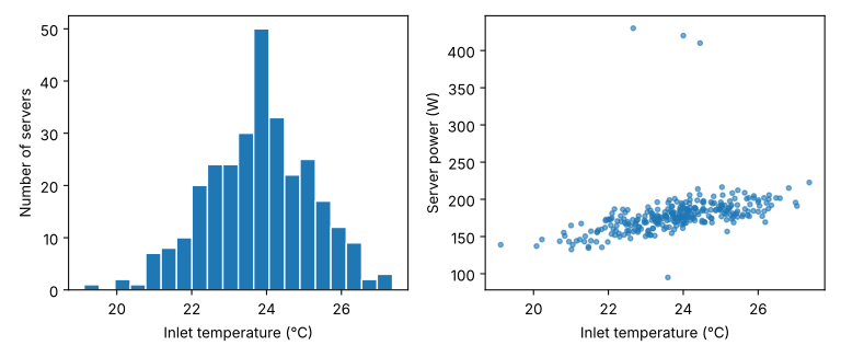
The summary statistics barely notice the odd readings: the mean and median differ by under 2 W. The scatter plot shows them instantly: three servers drawing over 400 W and one under 100 W, far from the band that every other server follows. Each could be a real fault (a stuck fan running at full speed, a server stuck in a reboot loop), a data error (watts and deciwatts confused, readings from the wrong device) or a different kind of machine. EDA does not decide which; it raises the question. Deleting outliers without understanding them is as dangerous as ignoring them.
The scatter plot also shows the main relationship: about 9 W more per degree of inlet temperature, as fans work harder. Setting alpha below 1 makes overlapping points visible, which matters when there are thousands of them.
Summary statistics are not enough
In 1973 the statistician Francis Anscombe published four small data sets that make this point unforgettable. All four have the same mean and variance of x and y, the same correlation, and the same best-fit line, to two decimal places. They could hardly look more different.
import numpy as np
import matplotlib.pyplot as plt

# Anscombe's quartet (F. J. Anscombe, 1973)
x = np.array([10, 8, 13, 9, 11, 14, 6, 4, 12, 7, 5])
x4 = np.array([8, 8, 8, 8, 8, 8, 8, 19, 8, 8, 8])
ys = [np.array([8.04, 6.95, 7.58, 8.81, 8.33, 9.96, 7.24, 4.26, 10.84, 4.82, 5.68]),
      np.array([9.14, 8.14, 8.74, 8.77, 9.26, 8.10, 6.13, 3.10, 9.13, 7.26, 4.74]),
      np.array([7.46, 6.77, 12.74, 7.11, 7.81, 8.84, 6.08, 5.39, 8.15, 6.42, 5.73]),
      np.array([6.58, 5.76, 7.71, 8.84, 8.47, 7.04, 5.25, 12.50, 5.56, 7.91, 6.89])]
xs = [x, x, x, x4]

fig, axes = plt.subplots(2, 2, figsize=(7, 5), sharex=True, sharey=True)
for i, (xi, yi, ax) in enumerate(zip(xs, ys, axes.flat), start=1):
    slope, intercept = np.polyfit(xi, yi, 1)
    r = np.corrcoef(xi, yi)[0, 1]
    print(f"set {i}: mean y {yi.mean():.2f}, var y {yi.var(ddof=1):.2f}, "
          f"r {r:.3f}, line y = {intercept:.2f} + {slope:.3f}x")
    ax.scatter(xi, yi)
    ax.plot([3, 20], [intercept + slope * 3, intercept + slope * 20], color="tab:red")
    ax.set_title(f"Set {i}")
fig.tight_layout()
fig.savefig("anscombe.png", dpi=150)set 1: mean y 7.50, var y 4.13, r 0.816, line y = 3.00 + 0.500x set 2: mean y 7.50, var y 4.13, r 0.816, line y = 3.00 + 0.500x set 3: mean y 7.50, var y 4.12, r 0.816, line y = 3.00 + 0.500x set 4: mean y 7.50, var y 4.12, r 0.817, line y = 3.00 + 0.500x
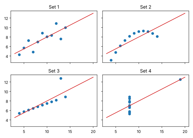
Set 1 is the only one where a straight line is a reasonable model. Set 2 is a smooth curve that a line misdescribes; set 3 is a perfect line spoiled by one outlier that drags the fit; and in set 4 a single point creates the whole relationship. A model trained on numbers alone would treat all four the same. The lesson applies directly to AI: plot the data before trusting any statistic or model fitted to it.
Relationships and correlation
Lesson 8 adds the statistical tools for judging whether the patterns found here are real: confidence intervals, tests and regression.
The Pearson correlation coefficient \(r\) measures how closely two variables follow a straight-line relationship, from −1 (perfectly decreasing) through 0 (no linear relationship) to +1 (perfectly increasing). Pandas computes it for every pair of numeric columns with df.corr(), and the resulting matrix is a quick map of which variables move together.
import numpy as np
import pandas as pd
import matplotlib.pyplot as plt

rng = np.random.default_rng(3)
n = 200
df = pd.DataFrame({"cpu_pct": rng.uniform(5, 95, n)})
df["power_w"] = 150 + 2.6 * df["cpu_pct"] + rng.normal(0, 15, n)
df["inlet_c"] = rng.normal(24, 1.2, n)
df["fan_rpm"] = 4000 + 25 * df["cpu_pct"] + 180 * (df["inlet_c"] - 24) + rng.normal(0, 150, n)
df["model"] = rng.choice(["Gen A", "Gen B", "Gen C"], n)
df.loc[df["model"] == "Gen C", "power_w"] -= 40          # newer servers draw less

print(df[["cpu_pct", "power_w", "inlet_c", "fan_rpm"]].corr().round(2))

fig, ax = plt.subplots(figsize=(6, 3.4))
groups = ["Gen A", "Gen B", "Gen C"]
ax.boxplot([df.loc[df["model"] == g, "power_w"] for g in groups])
ax.set_xticks([1, 2, 3], groups)
ax.set_ylabel("Server power (W)")
fig.tight_layout()
fig.savefig("by_model.png", dpi=150)
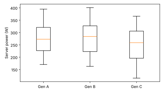
print(df.groupby("model")["power_w"].median().round(1))cpu_pct power_w inlet_c fan_rpm cpu_pct 1.00 0.93 0.14 0.93 power_w 0.93 1.00 0.16 0.87 inlet_c 0.14 0.16 1.00 0.43 fan_rpm 0.93 0.87 0.43 1.00 model Gen A 272.8 Gen B 283.9 Gen C 258.8 Name: power_w, dtype: float64
Reading the matrix needs care. Power and CPU load correlate at 0.93, as designed. Fan speed correlates with both CPU load (0.93) and power (0.87), but power does not drive the fans; CPU load drives both. Correlation does not show causation, and a model that predicts power from fan speed is relying on a proxy. Inlet temperature and CPU load show 0.14 even though the simulation made them completely independent: with 200 samples, small correlations of that size easily arise by chance. Treat weak correlations with scepticism until they are confirmed on more data.
The box plots show that the newer Gen C servers draw less power at the median, by about 14 to 25 W, but the boxes overlap heavily because CPU load varies so much within each group. To compare models fairly you would compare power at the same load, for example with a scatter plot of power against load coloured by model. That is the EDA loop: each picture raises the next question.
Worked problem
Choosing charts for a question
An operations team asks: (a) Has the average daily energy use of a data hall grown over the last year? (b) Which of 12 rows uses the most energy? (c) Do rows with hotter inlet temperatures have more server failures? (d) Is the distribution of rack power very uneven? Which chart answers each?
Show solution
- (a) A change over time: a line chart of daily energy against date, perhaps with a 30-day rolling mean to show the trend.
- (b) A comparison across categories: a bar chart of energy by row, sorted from largest to smallest, starting at zero.
- (c) A relationship between two numeric variables per row: a scatter plot of failures against mean inlet temperature, one point per row (only 12 points, so be cautious about conclusions).
- (d) A distribution: a histogram (or box plot) of power per rack.
Answer: Line chart; sorted bar chart; scatter plot; histogram. Matching the chart to the question is the most important plotting decision.
Scales, transformations and honesty
Some variables span many orders of magnitude: file sizes, request rates, model sizes, incomes. On a linear axis everything but the largest values is crushed against zero. A logarithmic axis (ax.set_yscale("log")) spaces powers of ten evenly and reveals the structure. Exponential growth, such as the compute used to train frontier AI models, appears as a straight line on a log scale, which makes the growth rate easy to read; always say clearly that the axis is logarithmic.
Charts can mislead, deliberately or not. Truncated bar axes exaggerate small differences; cherry-picked date ranges create trends; smoothing hides spikes; and colours that are hard to tell apart, especially red and green for the many people with colour-vision deficiency, hide categories. Use colour-blind-friendly palettes (Matplotlib's default "tab" colours and the viridis colour map are good choices), show the full context, and state how data was filtered or smoothed.
Beyond Matplotlib
Pandas DataFrames have a .plot method that calls Matplotlib with sensible defaults: df.plot(x="date", y="energy_kwh") draws a line chart in one line, and df["power_kw"].plot.hist() a histogram. Seaborn builds statistical charts (grouped box plots, pair plots of every variable against every other, regression lines with confidence bands) on top of Matplotlib with little code. Plotly and Altair create interactive charts for notebooks and web pages. All of them follow the same principles: right chart, labelled axes and units, honest scales.
Common mistakes
MistakeRelying on summary statistics without plotting the data.
InsteadPlot distributions and relationships first; Anscombe's quartet shows identical statistics can hide completely different data.
MistakeDeleting outliers automatically.
InsteadInvestigate each one: it may be a real fault, a data error or a different population.
MistakeReading correlation as causation.
InsteadA third variable can drive both (CPU load drives power and fan speed); test causal ideas with experiments or domain knowledge.
MistakeUnlabelled axes, missing units and no legend.
InsteadLabel every axis with its quantity and unit, and identify every series.
MistakeStarting a bar chart's axis above zero.
InsteadBars encode value by length, so their axis starts at zero; use a line or dot chart to show small differences.
Summary and key terms
- EDA (looking at the data before modelling) catches errors, suggests features and often answers the question directly.
- In Matplotlib, a Figure contains one or more Axes; create them with fig, ax = plt.subplots() and draw with ax methods.
- Label axes with units, add legends, keep gridlines light, use tight_layout and savefig.
- Line charts for change, histograms for distributions, scatter plots for relationships, bars for categories, box plots for group comparisons.
- Plots reveal outliers and patterns that summary statistics hide (Anscombe's quartet).
- Correlation measures linear association (−1 to +1), not causation; weak correlations can arise by chance.
- Use log scales for wide-ranging data and honest axes and colour-blind-friendly colours.
- pandas .plot, seaborn and interactive libraries build on the same principles.
- Exploratory data analysis (EDA)
- Examining data with plots and summaries to understand it before modelling.
- Figure
- In Matplotlib, the whole image, containing one or more Axes.
- Axes
- In Matplotlib, a single plot area with its axes, data and labels.
- Histogram
- A chart of how many values fall into each of a set of bins.
- Scatter plot
- A chart of points showing the relationship between two numeric variables.
- Box plot
- A summary of a distribution showing the median, the middle 50% (the box) and the range or outliers.
- Outlier
- A value far from the rest of the data, which may be an error or a genuine extreme.
- Distribution
- How the values of a variable are spread across their range.
- Skewed distribution
- A distribution with a longer tail on one side.
- Pearson correlation
- A measure from −1 to +1 of how closely two variables follow a straight-line relationship.
- Correlation matrix
- A table of correlation coefficients between every pair of variables.
- Confounding variable
- A third variable that influences two others, creating a correlation between them.
- Logarithmic scale
- An axis on which equal distances represent equal ratios, such as powers of ten.
- Anscombe's quartet
- Four data sets with nearly identical statistics but very different plots.
Practice problems
Work each problem on paper first, then reveal the answer to check.
Write the code to create a figure with two plots stacked vertically that share an x-axis.
Show answer
fig, (ax1, ax2) = plt.subplots(2, 1, sharex=True).
Which chart would you use to show how a server's power varies over a week, and which to show the spread of power across 1000 servers at one moment?
Show answer
A line chart against time for the week; a histogram (or box plot) for the spread across servers.
A histogram of request latencies has most values between 5 and 20 ms but a long tail to 2000 ms. What two things could you do to see the shape better?
Show answer
Use a logarithmic x-axis (or log-spaced bins), and report percentiles such as the median and 99th percentile rather than only the mean.
The mean of five readings [180, 182, 179, 181, 978] is 340. What is the median, and which better describes a typical reading?
Show answer
Median 181. The median, because the single 978 reading drags the mean far above every other value.
Two variables have a correlation of −0.85. Describe the relationship.
Show answer
A strong negative linear relationship: as one increases, the other tends to decrease, fairly consistently.
Ice cream sales and drowning incidents are positively correlated. Give the likely confounding variable.
Show answer
Hot weather (season), which increases both swimming and ice cream sales.
Why might fan speed be a poor input for a model that predicts server power, even though they correlate at 0.87?
Show answer
Fan speed is driven by CPU load and temperature rather than causing power; it is a proxy, and the relationship may change if fan control settings change. Using the underlying causes (load, temperature) is more robust.
What is wrong with a bar chart of energy by site whose y-axis runs from 980 to 1000 MWh?
Show answer
Bars encode values by length; truncating the axis makes a 2% difference look like several-fold. Start at zero or use a dot chart.
In Anscombe's set 3, one outlier pulls the fitted line. What would happen to the slope if that point were removed?
Show answer
The remaining points lie almost exactly on a line with a smaller slope (about 0.35), so the slope would fall and the fit would become nearly perfect.
List five things to check during EDA of a new data set.
Show answer
Any five of: shape and column meanings; data types; missing values; distributions and impossible values; outliers; duplicates; relationships between variables and with the target; differences between groups; changes over time or in measurement.
Lesson quiz · 5 questions
Score 60% or more to complete this lesson.
Create a free account to save your progress, take quizzes and earn a certificate.