Simulation, sampling and the bootstrap

Lesson 3 introduced NumPy arrays and seeded random number generators. This lesson puts them to work. Many questions in data and AI work are hard to answer with formulas but easy to answer by simulation: generate thousands or millions of random scenarios that follow the rules of the problem, and count what happens. The same idea, resampling the data you already have, gives honest uncertainty estimates for almost any statistic, and shuffling labels tests whether a difference between two groups could be chance. These techniques are the computational backbone of modern statistics and are used throughout machine learning, from estimating model accuracy to evaluating A/B tests.

Monte Carlo simulation

A Monte Carlo simulation estimates a quantity by random sampling. The recipe is always the same:

1. Describe one random scenario in code (one "trial").

2. Run many independent trials, ideally vectorized so that NumPy does them all at once.

3. Compute the fraction or average of interest across the trials.

4. Report the estimate together with its uncertainty, which shrinks as the number of trials grows.

The method is named after the casino in Monaco; it was developed by scientists at Los Alamos in the 1940s, who used early computers to simulate neutron transport.

A reliability question

A data hall has 20 cooling units and needs at least 19 running to remove the full heat load (an N+1 design). Each unit is unavailable 2% of the time, for failures or maintenance, independently of the others. What fraction of the time is the hall short of cooling?

import math
import numpy as np

n_units, p_down, needed = 20, 0.02, 19   # 20 cooling units, each down 2% of the time; 19 must run

rng = np.random.default_rng(42)
trials = 200_000
down = rng.random((trials, n_units)) < p_down      # True where a unit is down
short = (n_units - down.sum(axis=1)) < needed       # fewer than 19 running
print(f"Simulated P(capacity short): {short.mean():.5f}")

exact = 1 - sum(math.comb(n_units, k) * p_down**k * (1 - p_down)**(n_units - k) for k in range(2))
print(f"Exact binomial answer:       {exact:.5f}")
print("Hours per year short:", round(exact * 8760, 1))

Simulated P(capacity short): 0.06005
Exact binomial answer:       0.05990
Hours per year short: 524.7

The simulation builds a 200,000 × 20 Boolean array in one call, True wherever a unit is down, sums each row to count the units down, and averages the result. The exact answer comes from the binomial distribution: the hall is short when two or more units are down, so \(P = 1 - P(0) - P(1)\). The two agree to three decimal places.

The real power of simulation shows when the problem changes in ways that break the formula: units that fail together because they share an electrical feed, maintenance that is scheduled rather than random, repair times that vary. Each change is a few lines of code in the simulation and might be a research problem for the formula.

How accurate is a simulation?

A simulated probability is itself a random estimate. If the true probability is \(p\) and the simulation runs \(n\) independent trials, the standard error of the estimate is

and an approximate 95% confidence interval is the estimate ± 1.96 SE. The error shrinks with the square root of \(n\): to make it ten times smaller you need a hundred times more trials.

import numpy as np

rng = np.random.default_rng(7)
p_true = 0.0599
for n in [100, 10_000, 1_000_000]:
    hits = rng.random(n) < p_true
    est = hits.mean()
    se = np.sqrt(est * (1 - est) / n)
    print(f"n = {n:>9,}: estimate {est:.4f} +/- {1.96 * se:.4f}")

n =       100: estimate 0.0900 +/- 0.0561
n =    10,000: estimate 0.0577 +/- 0.0046
n = 1,000,000: estimate 0.0597 +/- 0.0005

With 100 trials the estimate of 0.09 is far from the true value of about 0.06 and its interval is wide; with a million it is within 0.0005. Always report the number of trials and the resulting uncertainty, and be especially careful with rare events: estimating a probability of one in a million needs many millions of trials, or special techniques such as importance sampling.

Sampling and the sampling distribution

The same logic applies to data. A data set is usually a sample from a larger population: 40 repair jobs out of all the repairs that will ever happen, 14 days of energy readings out of all possible days. Any statistic computed from the sample, a mean, a median, a model's accuracy, would come out differently with a different sample. The spread of a statistic across possible samples is its sampling distribution, and its standard deviation is the standard error. A result without some measure of this uncertainty can mislead badly, especially with small samples.

For a sample mean of \(n\) independent values with standard deviation \(s\), the classical formula is \(SE = s/\sqrt{n}\). But for medians, percentiles, ratios, correlations and model metrics, no simple formula exists, and for skewed data the formula's assumptions may fail. The bootstrap solves both problems.

The bootstrap

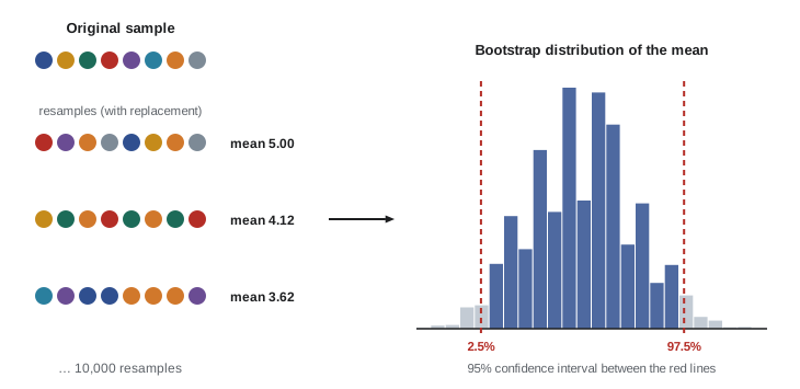
The bootstrap, introduced by Bradley Efron in 1979, treats the sample as a stand-in for the population. It draws many new samples of the same size from the data with replacement (so some values appear twice and others not at all), computes the statistic on each, and uses the spread of those values as the sampling distribution. The 2.5th and 97.5th percentiles of the bootstrap values give an approximate 95% confidence interval (the percentile method).

import numpy as np

rng = np.random.default_rng(3)
repair_h = np.round(rng.lognormal(mean=1.0, sigma=0.9, size=40), 1)   # 40 observed repair times, hours
print("Sample mean", round(repair_h.mean(), 2), "| median", np.median(repair_h), "| max", repair_h.max())

B = 10_000
idx = rng.integers(0, repair_h.size, size=(B, repair_h.size))   # resample with replacement
boot_means = repair_h[idx].mean(axis=1)
boot_medians = np.median(repair_h[idx], axis=1)

lo, hi = np.percentile(boot_means, [2.5, 97.5])
print(f"95% bootstrap CI for the mean:   {lo:.2f} to {hi:.2f} h")
lo, hi = np.percentile(boot_medians, [2.5, 97.5])
print(f"95% bootstrap CI for the median: {lo:.2f} to {hi:.2f} h")

Sample mean 4.89 | median 2.2 | max 54.1
95% bootstrap CI for the mean:   2.81 to 7.95 h
95% bootstrap CI for the median: 2.05 to 3.65 h

The repair times are strongly skewed: most jobs take a couple of hours, but one took 54. The mean is pulled up by the long jobs and is uncertain: its interval spans almost a factor of three. The median is more stable. The whole bootstrap takes one line of fancy indexing: repair_h[idx] builds a 10,000 × 40 array of resamples, and .mean(axis=1) computes all 10,000 means at once (Lesson 3).

The bootstrap is not magic. It cannot invent information the sample lacks: with very small samples, or for statistics such as the maximum that depend on rare extreme values, its intervals are unreliable. It also assumes the observations are independent; for time series, resample blocks of consecutive values instead of single points.

Comparing groups with a permutation test

A common question is whether a change made a difference: did a new fan control strategy reduce energy use, did a new model version reduce errors? If the two groups differ, how sure can we be that the difference is not chance?

A permutation test answers directly. If the change had no effect, the labels "old" and "new" are arbitrary, and shuffling them should produce differences as large as the observed one quite often. So we shuffle the labels many times, compute the difference each time, and count how often the shuffled difference is at least as large as the real one. That fraction is the p-value.

import numpy as np

rng = np.random.default_rng(11)
old = rng.normal(412, 18, size=14)   # daily cooling energy, MWh, old control
new = rng.normal(398, 18, size=14)   # after the new fan control
observed = old.mean() - new.mean()
print(f"Old {old.mean():.1f} MWh/day, new {new.mean():.1f} MWh/day, difference {observed:.1f}")

pooled = np.concatenate([old, new])
diffs = np.empty(20_000)
for i in range(diffs.size):
    perm = rng.permutation(pooled)
    diffs[i] = perm[:14].mean() - perm[14:].mean()
p_value = np.mean(diffs >= observed)
print(f"Permutation p-value (one-sided): {p_value:.4f}")

Old 415.5 MWh/day, new 390.5 MWh/day, difference 25.0
Permutation p-value (one-sided): 0.0003

Only about 3 in 10,000 shuffles produced a difference as large as the observed 25 MWh/day, so chance alone is a very unlikely explanation. Note what the test does and does not show. A small p-value says the difference is unlikely to be due to chance in the sampling; it does not say how big the effect really is (for that, give a bootstrap confidence interval for the difference) and it cannot rule out other causes, such as cooler weather in the second two weeks. Good experiments randomize which days get which treatment, or run both at the same time on comparable equipment, to rule such causes out.

Simulating a decision

Simulation also supports decisions under uncertainty. A team must decide how many spare optical transceivers to keep on site. Failures arrive randomly at a known average rate, and replacements take six weeks to arrive. Too few spares means waiting with a failed link; too many ties up money. Failures that occur independently at a constant rate follow a Poisson distribution, which NumPy samples directly.

import numpy as np

rng = np.random.default_rng(2026)
fleet, afr = 6000, 0.012          # transceivers in service, annual failure rate
lead_weeks = 6                    # weeks to receive replacements
mean_failures = fleet * afr * lead_weeks / 52
demand = rng.poisson(mean_failures, size=100_000)   # failures during one lead time

print(f"Expected failures per lead time: {mean_failures:.1f}")
for spares in [8, 10, 12, 14]:
    print(f"{spares:>2} spares on the shelf -> enough {np.mean(demand <= spares):.1%} of the time")

Expected failures per lead time: 8.3
 8 spares on the shelf -> enough 55.2% of the time
10 spares on the shelf -> enough 78.6% of the time
12 spares on the shelf -> enough 92.1% of the time
14 spares on the shelf -> enough 97.7% of the time

With about 8.3 expected failures per lead time, holding 8 spares is enough only about 55% of the time, while 12 covers about 92% and 14 about 98%. The team can now choose a service level explicitly and see what it costs. Holding the expected number of failures is a classic mistake: because demand varies, stocking exactly the average runs out about half the time.

Reproducibility and good practice

• Always create a generator with a seed (np.random.default_rng(seed)) and record the seed, so results can be reproduced exactly (Lesson 11).
• Check a simulation against a case with a known answer, as K6 did with the binomial formula, before trusting it on harder cases.
• Report the number of trials and the Monte Carlo uncertainty.
• Vectorize: generating one large array is usually tens to hundreds of times faster than a Python loop of single draws.
• State the assumptions, especially independence. Correlated failures, seasonal patterns and dependence between observations are where simulations and bootstraps most often go wrong.