
ACCT-102 · Lesson 11 of 12 · 30 min
Flexible budgets, standard costs and variance analysis
A budget earns its keep when actual results come in. Comparing actual results with the plan tells managers whether things went well or badly, but only if the comparison is fair. If Cedar Ridge sold more chairs than planned, its costs will naturally exceed the budget; that is not inefficiency. This lesson shows how flexible budgets make the comparison fair by adjusting the budget to the actual level of activity, how standard costs provide per-unit benchmarks, and how variance analysis splits each difference into a price part and a quantity part so that managers know where to look. It applies all of this to Cedar Ridge's chair line for the year just ended. ACCT-222 extends the analysis to sales mix, materials mix and yield variances.
Static and flexible budgets
A static budget is prepared for one planned level of activity, such as the 7,000 chairs in the master budget of lesson 10. A flexible budget shows what revenues and costs should have been for the actual level of activity, using the same cost formulas: variable costs at the budgeted rate per unit times actual units, and fixed costs at the budgeted amount. Comparing actual results with the flexible budget removes the effect of volume and isolates how well prices and costs were controlled.
| Cost formula | Static budget (7,000 chairs) | Flexible budget (7,100 chairs) |
|---|---|---|
| Sales at $180 per chair | $1,260,000 | $1,278,000 |
| Variable costs at $108 per chair | $756,000 | $766,800 |
| Contribution margin | $504,000 | $511,200 |
| Fixed costs | $360,000 | $360,000 |
| Operating income | $144,000 | $151,200 |
Last year Cedar Ridge sold 7,100 chairs, 100 more than planned, at an average price of $177 after discounts given to win a large retailer. Actual variable costs were $112.50 per chair ($106.30 of variable manufacturing cost and $6.20 of variable selling cost), and actual fixed costs were $366,000. Actual operating income was $91,950, $52,050 below the static budget. The flexible budget explains why.
# Flexible budget performance report (illustrative)
budget_units, actual_units = 7_000, 7_100
p_std, v_std, fixed_std = 180, 108, 360_000
p_act, v_act, fixed_act = 177, 112.50, 366_000

def income(units, p, v, fixed):
    return units * p - units * v - fixed

static = income(budget_units, p_std, v_std, fixed_std)
flexible = income(actual_units, p_std, v_std, fixed_std)
actual = income(actual_units, p_act, v_act, fixed_act)

print(f"Static budget income    ${static:>10,.0f}")
print(f"Flexible budget income  ${flexible:>10,.0f}")
print(f"Actual income           ${actual:>10,.0f}")
print(f"Sales-volume variance   ${flexible - static:>+10,.0f}")
print(f"Flexible-budget variance${actual - flexible:>+10,.0f}")
print(f"  Selling price         ${(p_act - p_std) * actual_units:>+10,.0f}")
print(f"  Variable costs        ${-(v_act - v_std) * actual_units:>+10,.0f}")
print(f" Fixed costs ${-(fixed_act - fixed_std):>+10,.0f}")Static budget income $ 144,000 Flexible budget income $ 151,200 Actual income $ 91,950 Sales-volume variance $ +7,200 Flexible-budget variance$ -59,250 Selling price $ -21,300 Variable costs $ -31,950 Fixed costs $ -6,000
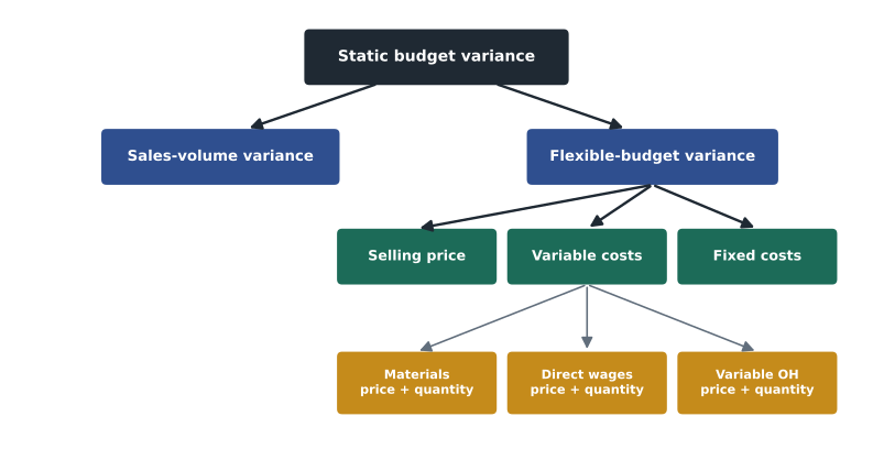
The static-budget variance of $52,050 unfavourable splits into two parts. The sales-volume variance of $7,200 favourable is the extra contribution margin from selling 100 more chairs than planned (100 × $72). The flexible-budget variance of $59,250 unfavourable is the difference between actual income and what income should have been at 7,100 chairs, and it is the part that reflects how well the business was run: $21,300 from lower selling prices (7,100 × $3), $31,950 from higher variable costs (7,100 × $4.50) and $6,000 from higher fixed costs. A variance is favourable (F) when it increases income relative to the budget and unfavourable (U) when it decreases income. Favourable does not automatically mean good, nor unfavourable bad: the price discounts may have been a deliberate trade for the extra volume.
Standard costs
To dig into the $31,950 of variable cost variance, managers need per-unit benchmarks for each input. A standard cost is the predetermined cost of making one unit under efficient operating conditions, built from a quantity standard (how much of each input should be used) and a price standard (how much each unit of input should cost). Standards are set with engineers, purchasing staff and supervisors, using time studies, past performance, supplier quotes and expected changes. Ideal standards assume perfect efficiency with no waste or downtime; practical (attainable) standards allow for normal waste, breaks and machine downtime. Most companies use practical standards, because ideal standards are rarely met and can discourage workers.
| Input | Standard quantity | Standard price | Standard cost per chair |
|---|---|---|---|
| Direct materials (hardwood) | 5 board feet | $12 per board foot | $60 |
| Direct labour | 1.5 hours | $20 per hour | $30 |
| Variable manufacturing overhead | 1.5 direct labour hours | $8 per hour | $12 |
| Fixed manufacturing overhead | 1.5 direct labour hours | $20 per hour | $30 |
| Total standard manufacturing cost | $132 |
Standard costs serve several purposes beyond variance analysis. They simplify bookkeeping, because inventory can be carried at standard; they support pricing and budgeting; and they communicate expectations to workers and supervisors. Lean manufacturers sometimes criticize standard costing for encouraging large batches and focusing on labour efficiency in automated plants, and many supplement it with non-financial measures such as defect rates and on-time delivery (lesson 12).
The general model for variable cost variances
Every variable input variance can be split into a price (rate or spending) variance and a quantity (usage or efficiency) variance. The price variance compares the actual price with the standard price for the actual quantity used. The quantity variance compares the actual quantity used with the standard quantity allowed for the actual output, valued at the standard price. The standard quantity allowed is what should have been used for the units actually produced.
In the formulas AP is the actual price per unit of input, SP the standard price, AQ the actual quantity used and SQ the standard quantity allowed for actual output. A positive result is unfavourable (actual exceeded standard) and a negative result favourable. Last year the chair line produced 7,000 chairs; it sold 7,100 by drawing 100 chairs from inventory. Production data were as follows.
| Actual production data (7,000 chairs produced) | Amount |
|---|---|
| Hardwood purchased and used | 36,400 board feet at $12.40 = $451,360 |
| Direct labour | 10,200 hours at $20.50 = $209,100 |
| Variable manufacturing overhead | $83,640 |
| Fixed manufacturing overhead | $219,000 |
| Standard quantities allowed for 7,000 chairs | 35,000 board feet; 10,500 direct labour hours |
# Standard cost variances for 7,000 chairs (illustrative)
output = 7_000
std = {"bf": 5, "bf_price": 12, "hours": 1.5, "rate": 20, "voh": 8}
act = {"bf": 36_400, "bf_price": 12.40, "hours": 10_200, "rate": 20.50, "voh_cost": 83_640}

sq_bf = output * std["bf"]
sq_hours = output * std["hours"]

def show(name, value):
    print(f"{name:<34}${abs(value):>9,.0f} {'U' if value > 0 else 'F'}")

show("Materials price variance", (act["bf_price"] - std["bf_price"]) * act["bf"])
show("Materials quantity variance", (act["bf"] - sq_bf) * std["bf_price"])
show("DL rate variance", (act["rate"] - std["rate"]) * act["hours"])
show("DL efficiency variance", (act["hours"] - sq_hours) * std["rate"])
show("Variable overhead spending variance", act["voh_cost"] - act["hours"] * std["voh"])
show("Variable overhead efficiency variance", (act["hours"] - sq_hours) * std["voh"])
total = (act["bf"] * act["bf_price"] + act["hours"] * act["rate"] + act["voh_cost"]
         - output * (std["bf"] * std["bf_price"] + std["hours"] * std["rate"] + std["hours"] * std["voh"]))
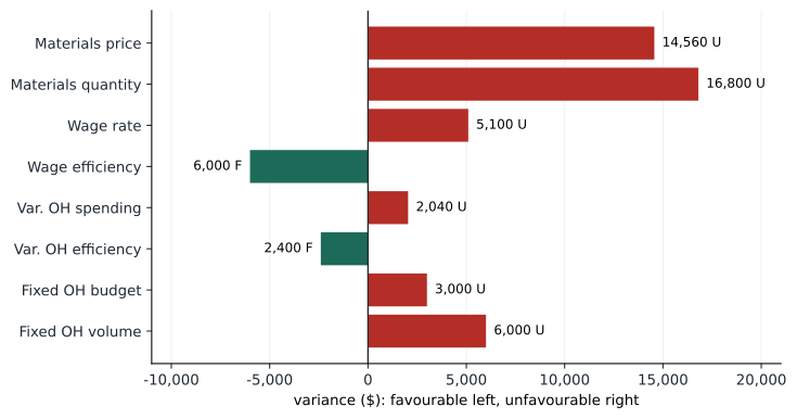
show("Total variable manufacturing variance", total)Materials price variance $ 14,560 U Materials quantity variance $ 16,800 U DL rate variance $ 5,100 U DL efficiency variance $ 6,000 F Variable overhead spending variance$ 2,040 U Variable overhead efficiency variance$ 2,400 F Total variable manufacturing variance$ 30,100 U
Interpreting materials variances
The materials price variance of $14,560 unfavourable says that hardwood cost 40 cents more per board foot than the standard. That is usually the purchasing manager's responsibility, but the cause may lie elsewhere: a general rise in lumber prices, a rush order that required air freight, or a decision to buy a better grade. The materials quantity variance of $16,800 unfavourable says that 1,400 more board feet were used than 7,000 chairs should need. That is usually the production supervisor's responsibility, but again the cause matters: inexperienced workers, poorly maintained saws, or poor-quality wood bought cheaply. Variances in different areas are often linked, which is why managers investigate before assigning blame.
Worked problem
Linked variances
Suppose the purchasing manager had instead bought a cheaper, knottier grade of hardwood at $11.50 per board foot and production then used 38,500 board feet. Compute the materials variances. What do they suggest?
Show solution
- Price variance = ($11.50 − $12.00) × 38,500 = $19,250 favourable.
- Quantity variance = (38,500 − 35,000) × $12 = $42,000 unfavourable.
- Net materials variance = $22,750 unfavourable.
- The favourable price variance is outweighed by extra waste: the cheaper grade cost more overall.
Answer: Purchasing looks good and production looks bad, but the root cause is the purchasing decision. Evaluating managers on single variances can encourage choices that hurt the company.
When materials are purchased in one period and used in another, the materials price variance is usually computed when the materials are purchased, on the quantity purchased, so that price problems are spotted early and raw materials inventory can be carried at standard. The quantity variance is computed on the quantity used.
Interpreting labour and variable overhead variances
The labour rate variance of $5,100 unfavourable arose because the average wage paid was 50 cents above standard, perhaps because of a negotiated wage increase not reflected in the standard, or because more senior workers were assigned to simple tasks. The labour efficiency variance of $6,000 favourable says the chairs took 300 fewer hours than the standard allows, perhaps because a new jig speeded assembly, or because the experienced workers who earned higher rates also worked faster. In that case the two labour variances are two sides of one staffing decision, netting to $900 favourable.
Variable overhead is applied on direct labour hours, so its efficiency variance moves with the labour efficiency variance: saving 300 hours also saved the variable overhead those hours would have caused, $2,400 favourable. The variable overhead spending variance of $2,040 unfavourable shows that, for the hours actually worked, more was spent on items such as power and supplies than the $8-per-hour rate allows. Investigating it means looking at the individual overhead items, comparing each with its flexible budget amount.
| Variance | Amount | Usually responsible | Possible causes |
|---|---|---|---|
| Materials price | $14,560 U | Purchasing | Market price rise, rush orders, grade choice, freight |
| Materials quantity | $16,800 U | Production | Waste, defective wood, untrained staff, poor maintenance |
| Labour rate | $5,100 U | Production and HR | Wage increases, overtime premiums, skill mix |
| Labour efficiency | $6,000 F | Production | Better methods or jigs, experienced staff, fewer delays |
| Variable overhead spending | $2,040 U | Production | Higher power or supply prices, waste of supplies |
| Variable overhead efficiency | $2,400 F | Production | Follows labour efficiency because overhead is applied on hours |
Fixed overhead variances
Fixed overhead does not change with output in the short run, so it is analysed differently. The budget (spending) variance compares actual fixed overhead with budgeted fixed overhead: $219,000 − $216,000 = $3,000 unfavourable. It is controllable in the usual sense and is investigated item by item. The production volume variance compares budgeted fixed overhead with the fixed overhead applied to production at the standard rate: applied overhead is 10,500 standard hours × $20 = $210,000, so the volume variance is $216,000 − $210,000 = $6,000 unfavourable.
The volume variance is not a measure of spending control. It arises because the plant produced 7,000 chairs rather than the 7,200 used to set the fixed overhead rate, so 200 chairs' worth of capacity cost ($6,000) was not absorbed into inventory. It is useful as a signal of unused capacity, which managers may be able to sell (lesson 9) or reduce, but treating it as a manager's failure can encourage overproduction, as lesson 8 warned. Together the two fixed overhead variances equal the underapplied fixed overhead of $9,000 ($219,000 actual against $210,000 applied).
# Fixed overhead variances (illustrative)
budget_foh, actual_foh = 216_000, 219_000
rate = budget_foh / 10_800            # $20 per hour at normal volume (7,200 chairs)
applied = 7_000 * 1.5 * rate          # standard hours allowed for actual output

print(f"Budget variance   ${actual_foh - budget_foh:,.0f} U")
print(f"Volume variance   ${budget_foh - applied:,.0f} U")
print(f"Underapplied fixed overhead ${actual_foh - applied:,.0f}")Budget variance $3,000 U Volume variance $6,000 U Underapplied fixed overhead $9,000
Management by exception and investigating variances
Managers cannot investigate every variance. Management by exception directs attention to variances that are large, either in dollars or as a percentage of the standard, that recur or trend in one direction, that involve controllable costs, or that are favourable by an amount that seems too good to be true (perhaps a quality corner being cut). Statistical control charts, borrowed from quality management (BUS-230 lesson 8), can distinguish random fluctuation from a real shift. The cost of investigating should be weighed against the expected benefit of correcting a problem.
Worked problem
Which variances deserve attention?
Cedar Ridge's controller investigates any variance above 5 per cent of the related flexible budget amount or above $10,000. Which of the year's variances qualify?
Show solution
- Materials flexible budget = 35,000 × $12 = $420,000; price variance $14,560 (3.5%) exceeds $10,000; quantity variance $16,800 (4.0%) exceeds $10,000.
- Labour flexible budget = 10,500 × $20 = $210,000; rate variance $5,100 (2.4%) and efficiency variance $6,000 (2.9%) are below both limits.
- Variable overhead flexible budget = $84,000; spending $2,040 (2.4%) is below both limits.
- Fixed overhead budget variance $3,000 (1.4%) is below both limits.
Answer: Investigate the two materials variances first; review the labour variances together because they may share a cause.
Standard costing systems often record variances in the ledger: inventory is debited at standard, and each variance has its own account, debited when unfavourable and credited when favourable. At year end, small variances are closed to cost of goods sold, and large ones may be prorated among inventories and cost of goods sold, as with under- or overapplied overhead in lesson 5. The detailed entries are covered in ACCT-222.
Common mistakes
MistakeComparing actual costs with the static budget when volume changed.
InsteadCompare with a flexible budget for the actual activity level.
MistakeComputing quantity variances with the actual output's budgeted quantity rather than the standard quantity allowed.
InsteadSQ is the standard quantity for the units actually produced.
MistakeTreating every favourable variance as good.
InsteadFavourable price variances may cause unfavourable quantity variances; look for links and quality effects.
MistakeBlaming the production manager for the volume variance.
InsteadThe volume variance reflects capacity use, not spending control.
MistakeInvestigating every variance regardless of size.
InsteadUse management by exception: focus on large, recurring or controllable variances.
Summary and key terms
- A flexible budget restates the plan for the actual level of activity.
- The static-budget variance splits into a sales-volume variance and a flexible-budget variance.
- Standard costs are built from quantity and price standards; practical standards are most common.
- Price variance = (AP − SP) × AQ; quantity variance = (AQ − SQ) × SP.
- Materials, labour and variable overhead variances often share causes and should be read together.
- Fixed overhead has a budget variance (controllable) and a volume variance (capacity use).
- Management by exception focuses investigation on significant, recurring or controllable variances.
- Static budget
- A budget prepared for one planned level of activity.
- Flexible budget
- A budget adjusted to the actual level of activity using cost formulas.
- Sales-volume variance
- The difference between flexible and static budget results caused by the volume of sales.
- Flexible-budget variance
- The difference between actual results and the flexible budget.
- Standard cost
- The predetermined cost of producing one unit under efficient conditions.
- Practical standard
- A standard achievable with normal waste and downtime.
- Price variance
- The difference between actual and standard price multiplied by the actual quantity.
- Quantity variance
- The difference between actual and standard quantity allowed multiplied by the standard price.
- Production volume variance
- Budgeted fixed overhead minus fixed overhead applied to actual output.
- Management by exception
- Focusing management attention on significant deviations from plan.
Practice problems
Work each problem on paper first, then reveal the answer to check.
A company planned 10,000 units with variable cost $15 each and fixed costs $50,000. Actual output was 11,000. What is the flexible budget total cost?
Show answer
11,000 × $15 + $50,000 = $215,000.
Actual materials: 23,000 kg at $4.10; standard 2 kg per unit at $4; 11,000 units made. Compute the price and quantity variances.
Show answer
Price $2,300 U; quantity (23,000 − 22,000) × $4 = $4,000 U.
Actual labour: 16,000 hours at $25.50; standard 1.5 hours per unit at $26; 11,000 units. Compute the rate and efficiency variances.
Show answer
Rate $8,000 F; efficiency (16,000 − 16,500) × $26 = $13,000 F.
Budgeted fixed overhead is $90,000 at 15,000 normal hours. Standard hours allowed are 16,500. Compute the volume variance.
Show answer
Rate $6; applied $99,000; volume variance $9,000 F.
Why might a favourable materials price variance be bad news?
Show answer
Cheaper, lower-quality materials may cause waste, rework or customer complaints.
Who is usually responsible for a labour efficiency variance?
Show answer
The production supervisor, though causes may lie with materials or equipment.
What does a sales-volume variance measure?
Show answer
The effect on income of selling more or fewer units than planned, at budgeted margins.
Give two criteria for deciding which variances to investigate.
Show answer
Size in dollars or percentage, recurrence or trend, controllability, apparent quality trade-offs.
Why does the variable overhead efficiency variance follow the labour efficiency variance at Cedar Ridge?
Show answer
Variable overhead is applied on direct labour hours, so hours saved also save overhead.
Change the variance program so 35,800 board feet were used at $12.40. What are the new materials variances?
Show answer
Price $14,320 U; quantity $9,600 U.
Lesson quiz · 5 questions
Score 60% or more to complete this lesson.
Create a free account to save your progress, take quizzes and earn a certificate.