
ACCT-102 · Lesson 4 of 12 · 32 min
Cost-volume-profit analysis
Cost-volume-profit (CVP) analysis studies how operating income responds to changes in selling prices, sales volume, variable costs, fixed costs and the mix of products sold. It is one of the most widely used tools in managerial accounting because it turns the cost behaviour of lesson 3 into quick answers to planning questions: how many units must we sell to break even, how many to earn a target profit, how much can sales fall before we lose money, and what happens to profit if we cut the price or automate a process. BUS-110 lesson 11 introduced break-even arithmetic for small businesses. This lesson extends it with after-tax targets, the margin of safety, operating leverage, multiple products, and a short look at uncertainty, using the Classic chair and the new trestle bench at Cedar Ridge.
The contribution margin and the CVP equation
Everything in CVP analysis flows from the contribution margin. Each Classic chair sells for $180 and has variable costs of $108 ($102 of variable manufacturing cost and $6 of variable selling cost), so each chair contributes $72 toward fixed costs and, once fixed costs are covered, toward profit. The contribution margin ratio expresses the same idea per dollar of sales: $72 ÷ $180 = 40 per cent. Every extra dollar of chair sales adds 40 cents of operating income, as long as fixed costs do not change.
In the equation p is the selling price per unit, v the variable cost per unit, Q the number of units sold and F total fixed costs. For the chair line, operating income = $72Q − $360,000. Every CVP formula in this lesson is a rearrangement of this one line.
| Item | Per chair | Ratio |
|---|---|---|
| Selling price | $180 | 100% |
| Variable costs | $108 | 60% |
| Contribution margin | $72 | 40% |
Break-even point
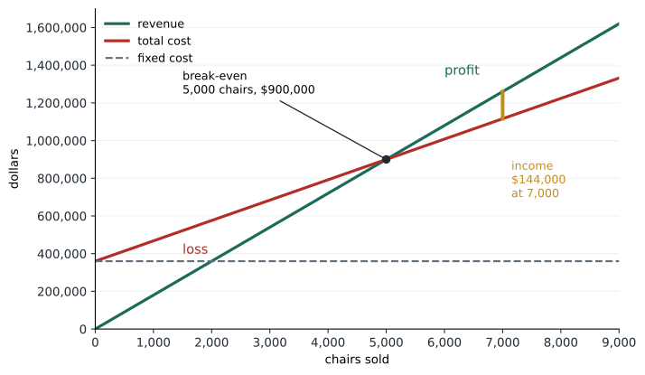
The break-even point is the sales level at which operating income is zero: contribution margin exactly covers fixed costs. In units, it is fixed costs divided by the contribution margin per unit. In sales dollars, it is fixed costs divided by the contribution margin ratio.
Worked problem
Break-even for the Classic chair
Find the chair line's break-even point in units and in sales dollars.
Show solution
- Break-even units = $360,000 ÷ $72 = 5,000 chairs.
- Break-even sales = $360,000 ÷ 0.40 = $900,000.
- Check: 5,000 × $180 = $900,000 of sales; contribution margin 5,000 × $72 = $360,000 equals fixed costs, so operating income is zero.
Answer: Break-even is 5,000 chairs, or $900,000 of sales.
The break-even point is a useful reference, but few businesses aim to break even. Its value is in showing how far the expected sales level sits above the danger line, and how sensitive that cushion is to changes in price and cost.
Target profit, before and after tax
To earn a target operating income, the contribution margin must cover fixed costs plus the target. Target units = (F + target operating income) ÷ (p − v). Managers often think in after-tax terms, because net income is what is left for owners. Since income tax is roughly a percentage of operating income, the after-tax target must be converted to a pre-tax target first: pre-tax income = after-tax income ÷ (1 − t), where t is the tax rate.
Worked problem
An after-tax profit target
Cedar Ridge's owners want the chair line to earn net income of $132,300 next year. Assume an illustrative combined federal and Ontario corporate tax rate of 26.5 per cent on the line's income. How many chairs must be sold?
Show solution
- Pre-tax income needed = $132,300 ÷ (1 − 0.265) = $132,300 ÷ 0.735 = $180,000.
- Required contribution margin = $360,000 + $180,000 = $540,000.
- Required units = $540,000 ÷ $72 = 7,500 chairs, or $1,350,000 of sales.
- Check: tax = 26.5% × $180,000 = $47,700; net income = $180,000 − $47,700 = $132,300.
Answer: 7,500 chairs. The tax rate is illustrative; actual rates depend on the province, the type of income and the small business deduction.
Taxes do not change the break-even point, because at break-even there is no income to tax. They only raise the sales needed to reach a given after-tax profit. The tax rates in this course are rounded for teaching; real effective rates depend on the jurisdiction, deductions and credits.
Margin of safety
The margin of safety is the amount by which expected (or actual) sales exceed break-even sales. It can be expressed in units, in dollars or as a percentage of expected sales. It answers the question every lender and owner asks: how far can sales fall before we start losing money?
Worked problem
Margin of safety
Expected sales are 7,000 chairs. Compute the margin of safety.
Show solution
- In units: 7,000 − 5,000 = 2,000 chairs.
- In dollars: 2,000 × $180 = $360,000.
- As a percentage: 2,000 ÷ 7,000 ≈ 28.6 per cent.
Answer: Sales can fall about 28.6 per cent before the chair line incurs a loss.
Operating leverage
Operating leverage describes how sensitive operating income is to changes in sales. A company with high fixed costs and low variable costs has high operating leverage: once fixed costs are covered, each extra sale adds a large contribution margin, so profits rise quickly in good times and fall quickly in bad times. The degree of operating leverage (DOL) at a given sales level is contribution margin divided by operating income. Multiplying the percentage change in sales by the DOL gives the percentage change in operating income.
# Classic chair: break-even, margin of safety and operating leverage (illustrative)
p, v, F = 180, 108, 360_000
cm = p - v
cmr = cm / p

def income(q):
    return cm * q - F

be_units = F / cm
expected = 7_000
mos = expected - be_units
dol = cm * expected / income(expected)

print(f"Break-even: {be_units:,.0f} chairs, ${F / cmr:,.0f} of sales")
print(f"Operating income at {expected:,}: ${income(expected):,}")
print(f"Margin of safety: {mos:,.0f} chairs ({mos / expected:.1%})")
print(f"Degree of operating leverage: {dol:.2f}")
new_q = expected * 1.10
print(f"10% more sales -> income ${income(new_q):,.0f} "
f"(+{income(new_q) / income(expected) - 1:.0%})")Break-even: 5,000 chairs, $900,000 of sales Operating income at 7,000: $144,000 Margin of safety: 2,000 chairs (28.6%) Degree of operating leverage: 3.50 10% more sales -> income $194,400 (+35%)
The DOL of 3.5 means that a 10 per cent rise in sales raises operating income by 35 per cent, from $144,000 to $194,400, and a 10 per cent fall cuts it by 35 per cent. DOL is not constant: it is very high just above break-even (where operating income is small) and falls as sales grow. Note also that the DOL is the reciprocal of the margin of safety percentage: 1 ÷ 0.286 ≈ 3.5. A small margin of safety and high operating leverage are two views of the same risk.
| Labour-intensive line | Automated line | |
|---|---|---|
| Variable cost per chair | $108 | $84 |
| Contribution margin per chair | $72 | $96 |
| Fixed costs | $360,000 | $528,000 |
| Break-even (chairs) | 5,000 | 5,500 |
| Operating income at 7,000 chairs | $144,000 | $144,000 |
| Degree of operating leverage at 7,000 | 3.50 | 4.67 |
| Operating income at 8,000 chairs | $216,000 | $240,000 |
| Operating income at 6,000 chairs | $72,000 | $48,000 |
The comparison shows the trade-off behind automation decisions. A CNC router and automated finishing line would cut variable cost per chair by $24 but add $168,000 a year of depreciation, maintenance and software. At the expected volume the two choices give the same profit; the indifference point is where they are equal. Above it the automated line wins, below it the current line wins. Whether to automate is therefore partly a bet on future volume and partly a capital budgeting question that FIN-201 lessons 7 to 9 address with discounted cash flows.
What-if analysis
Because the CVP equation is simple, managers can quickly test scenarios. The key discipline is to change only what the scenario changes and to recompute the contribution margin when prices or variable costs move.
# What-if scenarios for the Classic chair (illustrative)
def summary(label, p, v, F, q):
    cm = p - v
    oi = cm * q - F
    print(f"{label:<34} CM/unit {cm:>5.0f}  BE {F / cm:>6,.0f}  income {oi:>9,.0f}")

summary("Base plan", 180, 108, 360_000, 7_000)
summary("Hardwood +10% ($6 per chair)", 180, 114, 360_000, 7_000)
summary("Price -5%, volume +15%", 171, 108, 360_000, 8_050)
summary("Extra $40,000 advertising, +600 units", 180, 108, 400_000, 7_600)
summary("Commission cut by $2, volume -3%", 180, 106, 360_000, 6_790)Base plan CM/unit 72 BE 5,000 income 144,000 Hardwood +10% ($6 per chair) CM/unit 66 BE 5,455 income 102,000 Price -5%, volume +15% CM/unit 63 BE 5,714 income 147,150 Extra $40,000 advertising, +600 units CM/unit 72 BE 5,556 income 147,200 Commission cut by $2, volume -3% CM/unit 74 BE 4,865 income 142,460
Reading the results: a 10 per cent rise in hardwood prices cuts income by $42,000 and raises break-even to about 5,455 chairs. A 5 per cent price cut that lifts volume by 15 per cent raises income only slightly, because each chair now contributes $63 instead of $72; the volume gain barely outruns the margin loss. An advertising campaign is worthwhile only if it adds more than $40,000 ÷ $72 ≈ 556 chairs. Spreadsheets and short programs make these comparisons routine; the judgement lies in estimating how customers and suppliers will actually respond.
Multiple products and the sales mix
Most companies sell more than one product, each with its own contribution margin. CVP analysis then needs a sales mix assumption: the relative proportions in which products are sold. With a constant mix, the products can be treated as a single composite unit. Cedar Ridge plans to add a trestle bench that sells for $300 with variable costs of $195, a contribution margin of $105. Launching the bench adds $89,400 of fixed costs (a jig, a part-time finisher and catalogue space), bringing total fixed costs to $449,400. Managers expect to sell three chairs for every bench.
Worked problem
Break-even with a sales mix
With a 3:1 mix of chairs to benches and fixed costs of $449,400, find the break-even point.
Show solution
- A composite unit is 3 chairs and 1 bench.
- Composite contribution margin = 3 × $72 + 1 × $105 = $321.
- Break-even composite units = $449,400 ÷ $321 = 1,400.
- That is 1,400 × 3 = 4,200 chairs and 1,400 benches.
- In dollars: composite revenue = 3 × $180 + $300 = $840; break-even sales = 1,400 × $840 = $1,176,000. The weighted CM ratio is $321 ÷ $840 ≈ 38.2 per cent.
Answer: Break-even is 4,200 chairs and 1,400 benches, or $1,176,000 of sales, at the planned mix.
# Sales mix break-even and the effect of a mix shift (illustrative)
products = {"chair": (180, 108), "bench": (300, 195)}
F = 449_400

def breakeven(mix):
    cm = sum(n * (p - v) for (p, v), n in zip(products.values(), mix))
    rev = sum(n * p for (p, v), n in zip(products.values(), mix))
    comp = F / cm
    return comp, cm / rev

for mix in ((3, 1), (2, 1), (5, 1)):
    comp, cmr = breakeven(mix)
    plural = {"chair": "chairs", "bench": "benches"}
    units = ", ".join(f"{n * comp:,.0f} {plural[name]}" for name, n in zip(products, mix))
print(f"mix {mix[0]}:{mix[1]} weighted CMR {cmr:.1%} break-even: {units}")mix 3:1 weighted CMR 38.2% break-even: 4,200 chairs, 1,400 benches mix 2:1 weighted CMR 37.7% break-even: 3,610 chairs, 1,805 benches mix 5:1 weighted CMR 38.8% break-even: 4,832 chairs, 966 benches
The bench has a higher contribution margin per unit ($105) but a lower contribution margin ratio (35 per cent) than the chair (40 per cent). So shifting the mix toward benches lowers the weighted CM ratio and raises break-even sales dollars, even though each bench earns more dollars than each chair. When a constrained resource limits output, the right comparison changes again: lesson 9 shows how to rank products by contribution margin per unit of the scarce resource.
CVP assumptions and uncertainty
CVP analysis rests on simplifying assumptions: selling price and variable cost per unit are constant within the relevant range; costs can be split cleanly into fixed and variable; the sales mix is constant; and for manufacturers, production equals sales, so that inventory changes do not shift fixed costs between periods (lesson 8 relaxes this). When an assumption fails badly, for example when volume discounts lower the price at high volumes, the analysis must be refined or limited to a narrower range.
Real sales are uncertain. Managers can explore that uncertainty with sensitivity analysis (how much must a variable change to wipe out the profit?) or with simulation, which draws many possible sales outcomes from a probability distribution and reports the range of results.
# Simulating uncertain chair sales (illustrative, seeded)
import random
random.seed(102)
cm, F = 72, 360_000
results = [cm * max(0, random.gauss(7_000, 900)) - F for _ in range(10_000)]
results.sort()
loss = sum(r < 0 for r in results) / len(results)
print(f"Mean income        ${sum(results) / len(results):,.0f}")
print(f"5th percentile     ${results[500]:,.0f}")
print(f"95th percentile    ${results[9500]:,.0f}")
print(f"Probability of loss {loss:.1%}")Mean income $144,034 5th percentile $39,181 95th percentile $249,350 Probability of loss 1.1%
If annual sales are normally distributed around 7,000 chairs with a standard deviation of 900, the simulation suggests about a 1 per cent chance of a loss and a 90 per cent range of operating income from about $40,000 to $250,000. The assumed distribution is itself a judgement, so these figures are illustrations of the method rather than forecasts. Lesson 10 uses the same idea in budgeting.
Common mistakes
MistakeDividing fixed costs by the selling price to find break-even.
InsteadDivide by the contribution margin per unit, because variable costs must be covered first.
MistakeApplying the tax rate to the target units.
InsteadConvert after-tax income to pre-tax income first: NI ÷ (1 − t).
MistakeAssuming DOL is the same at every sales level.
InsteadDOL changes with volume; it is highest near break-even.
MistakeRanking products by contribution margin per unit when no resource is constrained and mix matters.
InsteadUse the weighted contribution margin for the expected mix; with a constraint, use CM per unit of the constraint (lesson 9).
MistakeUsing CVP results far outside the relevant range.
InsteadFixed costs step up and prices may change; re-estimate the model.
Summary and key terms
- CVP analysis links price, volume, variable cost, fixed cost and mix to operating income.
- Operating income = (p − v)Q − F; contribution margin per unit is p − v and the CM ratio is (p − v) ÷ p.
- Break-even units = F ÷ (p − v); break-even sales = F ÷ CMR.
- Target profit units add the pre-tax target to F; after-tax targets are divided by (1 − t).
- Margin of safety measures the cushion above break-even; DOL measures income sensitivity and equals 1 ÷ margin of safety %.
- Multiple-product CVP uses a composite unit or weighted CM ratio based on the sales mix.
- CVP assumptions limit its use; sensitivity analysis and simulation explore uncertainty.
- Cost-volume-profit analysis
- Analysis of how operating income changes with price, volume, costs and mix.
- Contribution margin ratio
- Contribution margin divided by sales.
- Break-even point
- The sales level at which operating income is zero.
- Target operating income
- The operating income a plan aims to achieve.
- Margin of safety
- The excess of expected or actual sales over break-even sales.
- Operating leverage
- The extent to which a cost structure relies on fixed rather than variable costs.
- Degree of operating leverage
- Contribution margin divided by operating income at a given sales level.
- Sales mix
- The relative proportions of products sold.
- Composite unit
- A bundle of products in the sales mix proportions, used for multi-product CVP.
- Indifference point
- The volume at which two cost structures give the same operating income.
Practice problems
Work each problem on paper first, then reveal the answer to check.
A product sells for $50 with variable costs of $30 and fixed costs of $80,000. Find break-even units and sales.
Show answer
4,000 units; $200,000.
For the same product, how many units give operating income of $40,000?
Show answer
(80,000 + 40,000) ÷ 20 = 6,000 units.
With a 25 per cent tax rate, how many units give net income of $45,000?
Show answer
Pre-tax $60,000; (80,000 + 60,000) ÷ 20 = 7,000 units.
Expected sales are 5,000 units. Compute the margin of safety percentage and the DOL.
Show answer
MOS 1,000 ÷ 5,000 = 20%; operating income $20,000; DOL = 100,000 ÷ 20,000 = 5.
Using that DOL, what happens to income if sales rise 8 per cent?
Show answer
Income rises 40 per cent, to $28,000.
For the chair line, how many extra chairs must a $25,000 trade show produce to pay for itself?
Show answer
25,000 ÷ 72 ≈ 348 chairs.
Find the indifference point between the labour-intensive and automated chair lines.
Show answer
72Q − 360,000 = 96Q − 528,000; Q = 7,000 chairs.
With a 2:1 chair-to-bench mix and fixed costs of $449,400, find break-even in composite units.
Show answer
Composite CM = 2 × 72 + 105 = $249; 449,400 ÷ 249 ≈ 1,805 composites (3,610 chairs and 1,805 benches).
Why does a shift toward benches raise break-even sales dollars?
Show answer
Benches have a lower CM ratio (35%) than chairs (40%), lowering the weighted ratio.
Change the simulation's standard deviation to 1,500. What happens to the probability of loss and why?
Show answer
It rises (to roughly 9–10 per cent) because outcomes below 5,000 chairs become more likely.
Lesson quiz · 5 questions
Score 60% or more to complete this lesson.
Create a free account to save your progress, take quizzes and earn a certificate.