
ACCT-102 · Lesson 3 of 12 · 26 min
Cost behaviour and estimation
To plan, a manager must predict what costs will be at the activity level expected next period. To control, she must know what costs should have been at the activity level actually achieved. Both require an understanding of cost behaviour: how a cost changes in total as an activity, such as units produced, labour hours or kilometres driven, changes. Lesson 2 introduced variable, fixed and mixed costs. This lesson looks more closely at the patterns costs follow, the relevant range within which those patterns hold, and three practical ways to estimate a cost's fixed and variable components from data: account analysis, the high–low method and least-squares regression. It ends with the contribution margin income statement, the report format that makes cost behaviour visible and that lesson 4 relies on.
Cost drivers and the relevant range
A cost driver is the activity that causes a cost to change. For hardwood, the driver is chairs produced. For machine maintenance, it may be machine hours. For the cost of processing customer orders, it may be the number of orders. Choosing the right driver matters: a cost that looks unpredictable against units may be closely related to batches or set-ups. Managers usually start with volume-based drivers such as units or labour hours, and lesson 7 adds activity-based drivers.
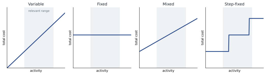
Cost behaviour patterns hold only within a relevant range of activity, the band within which the company expects to operate and within which the assumed relationships are reasonable. Cedar Ridge's chair line can make between about 5,000 and 8,500 chairs a year with its present building, equipment and supervisors. Within that range, fixed manufacturing overhead is $216,000. Beyond it, the company would need another shift supervisor, more equipment or a larger building, and the fixed cost would jump. Outside the range, the economics are different and the usual formulas should not be trusted.
Common cost behaviour patterns
| Pattern | Behaviour in total | Behaviour per unit | Cedar Ridge example |
|---|---|---|---|
| Variable | Rises in proportion to activity | Constant | Hardwood: $60 per chair |
| Fixed | Constant within the relevant range | Falls as activity rises | Factory lease, depreciation |
| Mixed (semivariable) | Fixed base plus variable part | Falls, but not to zero | Maintenance and utilities |
| Step-variable | Rises in small steps | Fluctuates | Part-time finishers hired per 200 chairs a month |
| Step-fixed | Constant over wide bands, then jumps | Falls within each band | One supervisor per shift of up to 4,500 chairs |
| Curvilinear | Changes at a changing rate | Varies | Overtime and congestion near capacity |
Committed fixed costs arise from long-term decisions about capacity, such as buildings, equipment and key managers; they cannot be cut quickly without harming the business. Discretionary fixed costs result from annual management decisions, such as advertising, training and research; they can be adjusted more readily, though cutting them may hurt the future. Distinguishing the two helps managers know where savings are possible in a downturn.
Economists draw total cost curves that bend, because variable cost per unit falls at first as workers specialize and later rises as the plant becomes congested. Accountants usually assume straight lines. The two views are reconciled by the relevant range: over the band where a company actually operates, the economist's curve is close to a straight line, so the linear approximation is good enough for planning.
Mixed costs and the cost formula
A mixed cost can be written as a cost formula: total cost = fixed cost + (variable cost per unit of driver × activity), or Y = a + bX. Here Y is total cost, a is the fixed component (the intercept), b is the variable cost per unit of the driver (the slope) and X is the activity level. Once a and b are estimated, the formula predicts the cost at any activity within the relevant range.
Cedar Ridge's factory maintenance and utilities cost is a typical mixed cost. Part of it is fixed: basic electricity for lighting and heat, a maintenance contract, the base charge on the gas bill. Part varies with machine use: power for the saws, router and dust collectors, and wear parts. Managers want to know the split to budget the cost for next year and to judge whether a month's bill was reasonable.
Method 1: account analysis
The simplest method is account analysis: an experienced accountant reviews each account in the ledger and classifies it as variable, fixed or mixed, using judgement and knowledge of the operation. Hardwood is variable; the factory lease is fixed; the electricity bill is mixed and might be split using the utility's tariff, which shows the fixed service charge and the energy charge per kilowatt-hour. Account analysis is quick and uses knowledge that statistical methods lack, but it is subjective and may miss changes in behaviour.
The engineering approach is a more rigorous variation: engineers study the process and estimate how much of each input should be used per unit, for example by timing operations or measuring the board feet a chair design requires. It is the basis for standard costs (lesson 11) and works even when there is no past data, such as for a new product.
Method 2: the high–low method
The high–low method estimates the cost formula from just two observations: the periods with the highest and lowest activity. The change in cost between them is assumed to be caused entirely by the change in activity, so the variable rate is the change in cost divided by the change in activity. The fixed component is then the total cost at either point minus the variable part.
| Month | Machine hours | Maintenance and utilities ($) |
|---|---|---|
| Jan | 1,800 | 21,400 |
| Feb | 2,400 | 24,800 |
| Mar | 2,100 | 22,900 |
| Apr | 3,000 | 28,000 |
| May | 2,700 | 26,500 |
| Jun | 2,200 | 23,700 |
| Jul | 1,950 | 22,300 |
| Aug | 2,600 | 25,400 |
| Sep | 2,850 | 27,300 |
| Oct | 2,300 | 24,100 |
| Nov | 2,050 | 22,200 |
| Dec | 2,550 | 25,300 |
Worked problem
High–low estimate
Use the high and low activity months from the table to estimate the cost formula, and predict the cost for a month with 2,500 machine hours.
Show solution
- Choose the months by activity, not by cost: high is April (3,000 hours, $28,000); low is January (1,800 hours, $21,400).
- Variable rate b = (28,000 − 21,400) ÷ (3,000 − 1,800) = 6,600 ÷ 1,200 = $5.50 per machine hour.
- Fixed cost a = 28,000 − 5.50 × 3,000 = 28,000 − 16,500 = $11,500 per month.
- Check with the low point: 11,500 + 5.50 × 1,800 = 11,500 + 9,900 = $21,400.
- Prediction at 2,500 hours: 11,500 + 5.50 × 2,500 = $25,250.
Answer: Cost = $11,500 per month + $5.50 per machine hour; predicted cost at 2,500 hours is $25,250.
The high–low method is easy, but it rests on only two points, and those two are by definition the most extreme. If either month was unusual, such as a month with a large one-off repair, the estimate will be distorted. Always pick the high and low points by the activity measure, never by cost, and check a scatter plot first to make sure neither point is an outlier.
Method 3: least-squares regression
Least-squares regression uses all the observations. It fits the straight line that minimizes the sum of the squared vertical distances between the observed costs and the line. Spreadsheets and statistical software do the arithmetic, but the formulas are short enough to code directly. The slope b equals the covariance of activity and cost divided by the variance of activity, and the intercept a equals mean cost minus b times mean activity. The coefficient of determination, R², measures the proportion of the variation in cost explained by the activity; values close to 1 mean the driver explains most of the variation.
# Estimate the maintenance cost formula two ways (illustrative data)
import statistics as st

hours = [1800, 2400, 2100, 3000, 2700, 2200, 1950, 2600, 2850, 2300, 2050, 2550]
cost  = [21400, 24800, 22900, 28000, 26500, 23700, 22300, 25400, 27300, 24100, 22200, 25300]

# High-low: pick extremes by activity
hi, lo = hours.index(max(hours)), hours.index(min(hours))
b_hl = (cost[hi] - cost[lo]) / (hours[hi] - hours[lo])
a_hl = cost[hi] - b_hl * hours[hi]

# Least squares
mx, my = st.mean(hours), st.mean(cost)
b_ls = sum((x - mx) * (y - my) for x, y in zip(hours, cost)) / sum((x - mx) ** 2 for x in hours)
a_ls = my - b_ls * mx
r2 = st.correlation(hours, cost) ** 2

for name, a, b in (("High-low", a_hl, b_hl), ("Regression", a_ls, b_ls)):
    print(f"{name:<11} fixed ${a:,.0f}/month, variable ${b:.2f}/hour, "
          f"cost at 2,500 h ${a + b * 2500:,.0f}")
print(f"R-squared {r2:.3f}")High-low fixed $11,500/month, variable $5.50/hour, cost at 2,500 h $25,250 Regression fixed $11,175/month, variable $5.61/hour, cost at 2,500 h $25,193 R-squared 0.989
Regression puts the fixed cost at about $11,175 a month and the variable rate at about $5.61 per machine hour, and R² of about 0.99 shows that machine hours explain almost all the month-to-month variation. The two methods give predictions within about $60 of each other at 2,500 hours, because these invented data happen to be well behaved. Real data are noisier, and regression is then clearly better, because it is not hostage to two extreme months. Python's statistics module also provides a linear_regression function that returns the same slope and intercept.
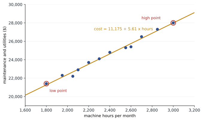
Three cautions apply to any estimate. First, the intercept is an estimate of fixed cost within the relevant range; it is not the cost the company would incur at zero activity, which was never observed. Second, check that the driver makes economic sense: a high R² between two unrelated series is a coincidence, not a cost formula. Third, adjust past data for known changes, such as a new utility rate, before relying on it. Regression with several drivers, such as machine hours and number of set-ups, is possible and is covered in ACCT-341.
| Method | Strengths | Weaknesses |
|---|---|---|
| Account analysis | Fast; uses managers' knowledge | Subjective; may misclassify mixed costs |
| Engineering | Works without history; basis for standards | Time-consuming; may ignore real-world inefficiency |
| High–low | Simple; needs only two data points | Ignores most data; distorted by outliers |
| Scatter plot (visual fit) | Reveals outliers and patterns | Line placement is subjective |
| Least-squares regression | Uses all data; gives R² and objective fit | Needs enough reliable data; can mislead if the driver is wrong |
The contribution margin income statement
Once costs are separated into variable and fixed, they can be reported in contribution format. The contribution margin income statement subtracts all variable costs, both manufacturing and selling, from sales to give the contribution margin, the amount available to cover fixed costs and then provide profit. It then subtracts all fixed costs. The traditional (functional) income statement used in external reporting, by contrast, subtracts cost of goods sold, which mixes variable and fixed manufacturing costs, to give gross margin, and then subtracts selling and administrative expenses, which also mix variable and fixed costs.
# Classic chair line: traditional versus contribution format (illustrative)
units, price = 7_000, 180
v_mfg, v_sell = 102, 6                 # variable manufacturing and selling per chair
f_mfg, f_sa = 216_000, 144_000         # fixed manufacturing and fixed S&A
sales = units * price

# Contribution format
vc = units * (v_mfg + v_sell)
cm = sales - vc
oi_cm = cm - f_mfg - f_sa

# Traditional format (assumes production equals sales)
cogs = units * v_mfg + f_mfg
gross = sales - cogs
sa = units * v_sell + f_sa
oi_trad = gross - sa

print(f"Contribution: sales {sales:,} - variable {vc:,} = CM {cm:,}; - fixed {f_mfg + f_sa:,} = {oi_cm:,}")
print(f"Traditional:  sales {sales:,} - COGS {cogs:,} = gross {gross:,}; - S&A {sa:,} = {oi_trad:,}")
print(f"CM ratio {cm / sales:.0%}; operating income identical: {oi_cm == oi_trad}")Contribution: sales 1,260,000 - variable 756,000 = CM 504,000; - fixed 360,000 = 144,000 Traditional: sales 1,260,000 - COGS 930,000 = gross 330,000; - S&A 186,000 = 144,000 CM ratio 40%; operating income identical: True
Both statements show the same operating income of $144,000 when production equals sales; lesson 8 shows what happens when it does not. What differs is the information they reveal. The contribution format shows at a glance that each additional $1 of sales adds 40 cents of contribution margin, which is exactly what a manager needs to predict the effect of changes in volume. The traditional format's gross margin of $330,000 says nothing about how costs will move if volume changes, because it buries $216,000 of fixed overhead inside cost of goods sold.
| Line | Traditional format | Contribution format |
|---|---|---|
| Sales | $1,260,000 | $1,260,000 |
| Cost of goods sold / variable costs | $930,000 | $756,000 |
| Gross margin / contribution margin | $330,000 | $504,000 |
| Selling and admin / fixed costs | $186,000 | $360,000 |
| Operating income | $144,000 | $144,000 |
Common mistakes
MistakeChoosing high and low points by cost.
InsteadChoose them by activity, then read off the related costs.
MistakeTreating the intercept as the cost at zero activity.
InsteadIt is the fixed component within the relevant range; zero activity was never observed.
MistakeUsing cost formulas far outside the relevant range.
InsteadBeyond the range fixed costs step up and variable rates may change; re-estimate.
MistakeAccepting a high R² without checking the driver makes economic sense.
InsteadCorrelation is not causation; pick drivers that plausibly cause the cost.
MistakeUsing the traditional income statement to predict profit at a new volume.
InsteadUse the contribution format, which separates variable from fixed costs.
Summary and key terms
- A cost driver is the activity that causes a cost; behaviour patterns hold within a relevant range.
- Patterns include variable, fixed, mixed, step-variable, step-fixed and curvilinear costs.
- A mixed cost can be expressed as Y = a + bX.
- Account analysis and engineering studies rely on judgement and process knowledge.
- The high–low method uses the highest and lowest activity points; it is simple but sensitive to outliers.
- Least-squares regression uses all data and reports R² as a measure of fit.
- The contribution margin income statement separates variable and fixed costs and supports volume-based planning.
- Cost driver
- An activity that causes a cost to be incurred.
- Relevant range
- The band of activity within which assumed cost behaviour holds.
- Mixed cost
- A cost with both fixed and variable components.
- Step-fixed cost
- A cost that is constant over a wide range of activity and then jumps to a new level.
- Committed fixed cost
- A fixed cost arising from long-term capacity decisions.
- Discretionary fixed cost
- A fixed cost set by periodic management decisions, such as advertising.
- High–low method
- A method of estimating fixed and variable cost from the highest and lowest activity observations.
- Least-squares regression
- A statistical method that fits the line minimizing the sum of squared errors.
- Coefficient of determination
- R²: the proportion of variation in a cost explained by the driver.
- Contribution margin
- Sales minus all variable costs; the amount available to cover fixed costs and profit.
Practice problems
Work each problem on paper first, then reveal the answer to check.
A cost was $18,000 at 4,000 units and $24,000 at 7,000 units. Estimate the cost formula.
Show answer
b = 6,000 ÷ 3,000 = $2 per unit; a = 18,000 − 8,000 = $10,000.
Using that formula, predict cost at 5,500 units.
Show answer
10,000 + 2 × 5,500 = $21,000.
Classify a supervisor hired for each 4,500 chairs per shift.
Show answer
Step-fixed cost.
Why might regression be preferred to high–low?
Show answer
It uses all observations and is not distorted by one unusual extreme point.
A regression has R² = 0.35. What does that suggest?
Show answer
The driver explains only 35 per cent of cost variation; look for a better driver or more drivers.
Give one committed and one discretionary fixed cost for Cedar Ridge.
Show answer
Committed: factory lease or depreciation; discretionary: advertising or training.
Sales $500,000, variable costs $300,000, fixed costs $150,000. Prepare a contribution format summary.
Show answer
CM $200,000 (40 per cent); operating income $50,000.
Why does gross margin not show how profit changes with volume?
Show answer
Cost of goods sold mixes fixed and variable costs.
Edit the program to predict the cost at 3,200 machine hours. Should you trust it?
Show answer
About $29,100 by either method, but 3,200 is above the highest observed level, so treat it with caution.
What is the difference between a cost driver and a cost object?
Show answer
A cost object is what we want to cost; a driver is the activity that causes the cost.
Lesson quiz · 5 questions
Score 60% or more to complete this lesson.
Create a free account to save your progress, take quizzes and earn a certificate.