
PYTH-201 · Lesson 9 of 12 · 26 min
Trees and binary search trees
▶ Video coming soon A video version of this lesson is on the way.
Ridgeline's online shop organizes its products into categories: Coffee splits into Single Origin, Blends and Decaf; Single Origin splits again by region; Equipment splits into Brewers, Grinders and Mugs. Each category has one parent and any number of children. This branching shape is a tree, and trees are everywhere in computing: folders on a disk, the structure of a web page, an organization chart, the decisions in a game and the indexes inside databases.
This lesson introduces tree vocabulary and the standard ways to visit every node of a tree, then focuses on the binary search tree, a tree that keeps keys in sorted order so that searching, inserting and listing in order are all efficient. You will build one, see why its speed depends on its shape, and learn how balanced trees keep that shape under control.
Tree vocabulary
A tree is made of nodes connected by edges, with no loops. The single node at the top is the root. Every other node has exactly one parent, the node directly above it, and may have children below it. Nodes with no children are leaves. The depth of a node is the number of edges from the root to it, and the height of a tree is the greatest depth of any node. Any node, together with everything below it, forms a subtree, which is itself a tree: the recursive structure that makes recursion, from lesson 6, the natural way to process trees.
In Python, a general tree node can hold a value and a list of children. Ridgeline's category tree fits that shape directly.
class Category:
    def __init__(self, name, children=None):
        self.name = name
        self.children = children or []

shop = Category("Shop", [
    Category("Coffee", [
        Category("Single Origin", [Category("Africa"), Category("Americas"), Category("Asia")]),
        Category("Blends"),
        Category("Decaf"),
    ]),
    Category("Equipment", [Category("Brewers"), Category("Grinders"), Category("Mugs")]),
])

def show(node, depth=0):
    print("  " * depth + node.name)
    for child in node.children:
        show(child, depth + 1)

def height(node):
    if not node.children:
        return 0                                   # a leaf has height 0
    return 1 + max(height(c) for c in node.children)

show(shop)
print("height:", height(shop))Shop
Coffee
Single Origin
Africa
Americas
Asia
Blends
Decaf
Equipment
Brewers
Grinders
Mugs
height: 3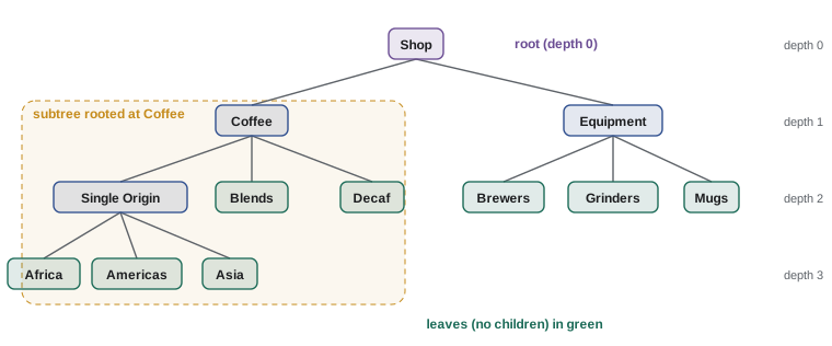
Traversals
Visiting every node of a tree is called a traversal, and the order matters. In a preorder traversal, you visit a node before its children, which is how the category tree was printed: each heading appears above its contents. In a postorder traversal, you visit the children first and the node afterward, which suits calculations that need the answers from below, such as a category's total product count or a folder's total size. A level-order traversal visits the tree one depth at a time, root first, using the queue from lesson 3.
from collections import deque

class Node:
    def __init__(self, name, children=()):
        self.name, self.children = name, list(children)

tree = Node("Shop", [Node("Coffee", [Node("Blends"), Node("Decaf")]),
                     Node("Equipment", [Node("Mugs")])])

def preorder(n):
    yield n.name
    for c in n.children:
        yield from preorder(c)

def postorder(n):
    for c in n.children:
        yield from postorder(c)
    yield n.name

def level_order(root):
    queue = deque([root])
    while queue:
        n = queue.popleft()
        yield n.name
        queue.extend(n.children)

print("pre:  ", list(preorder(tree)))
print("post: ", list(postorder(tree)))
print("level:", list(level_order(tree)))pre: ['Shop', 'Coffee', 'Blends', 'Decaf', 'Equipment', 'Mugs'] post: ['Blends', 'Decaf', 'Coffee', 'Mugs', 'Equipment', 'Shop'] level: ['Shop', 'Coffee', 'Equipment', 'Blends', 'Decaf', 'Mugs']
Each traversal visits every node exactly once, so all three are O(n). The recursive versions use one stack frame per level, so their extra space is O(h) for a tree of height h; the level-order version holds at most one level's worth of nodes in its queue. The yield from statement, from PYTH-102, hands on every value produced by the recursive call, which turns these traversals into generators that can be used in loops and comprehensions.
Try it yourself
Count products in each category
Category nodes have a name, a list of children, and a whole number products (products listed directly in that category). Write total_products(node) that returns the number of products in the category and all of its subcategories, at every level.
This is a postorder calculation: add up the totals of the children, then add the node's own products.
def total_products(node):
    return node.products + len(node.children)

print(total_products(shop))
Binary search trees
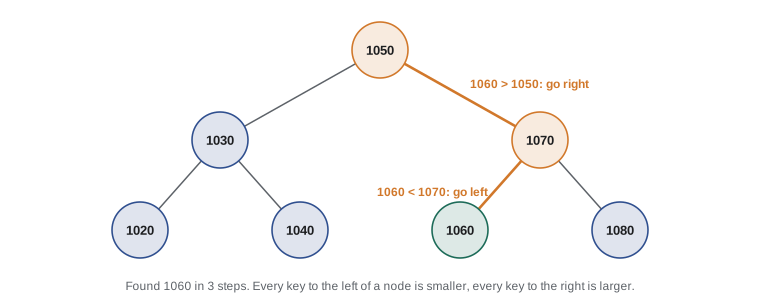
A binary tree is a tree in which every node has at most two children, called left and right. A binary search tree (BST) adds one rule, the search property: for every node, every key in its left subtree is smaller than the node's key, and every key in its right subtree is larger. That rule turns the tree into a decision structure. To find a key, start at the root and compare: if the key is smaller, go left; if larger, go right; if equal, you have found it. Each step moves one level down, so a search costs O(h), the height of the tree.
Inserting follows the same path: walk down as if searching, and when you fall off the tree, attach a new node in that empty spot. Because every insertion lands where a search would look for it, the search property is kept automatically. Jordan uses a BST to index the shop's order numbers as they arrive.
class Node:
    __slots__ = ("key", "value", "left", "right")
    def __init__(self, key, value):
        self.key, self.value, self.left, self.right = key, value, None, None

class BST:
    def __init__(self):
        self.root, self.size = None, 0

    def insert(self, key, value):
        if self.root is None:
            self.root = Node(key, value); self.size += 1; return
        node = self.root
        while True:
            if key == node.key:
                node.value = value; return          # existing key: update
            side = "left" if key < node.key else "right"
            child = getattr(node, side)
            if child is None:
                setattr(node, side, Node(key, value)); self.size += 1; return
            node = child

    def get(self, key):
        node, steps = self.root, 0
        while node is not None:
            steps += 1
            if key == node.key:
                return node.value, steps
            node = node.left if key < node.key else node.right
        return None, steps

orders = BST()
for order_id, total in [(1050, 41.5), (1030, 18.5), (1070, 64.25), (1020, 22.0),
                        (1040, 9.5), (1060, 37.0), (1080, 19.75)]:
    orders.insert(order_id, total)
print(orders.size, orders.get(1060), orders.get(1045))7 (37.0, 3) (None, 3)
In-order traversal: sorted for free
A third traversal is special to binary trees. An in-order traversal visits the left subtree, then the node, then the right subtree. In a binary search tree, the search property means this produces the keys in sorted order: everything smaller comes out before the node, and everything larger after it. So a BST gives you both fast lookup and a sorted listing, and it can find the minimum (keep going left), the maximum (keep going right) and every key in a range by skipping subtrees that cannot contain it.
class Node:
    def __init__(self, key, left=None, right=None):
        self.key, self.left, self.right = key, left, right

root = Node(1050, Node(1030, Node(1020), Node(1040)), Node(1070, Node(1060), Node(1080)))

def in_order(node):
    if node:
        yield from in_order(node.left)
        yield node.key
        yield from in_order(node.right)

def keys_between(node, low, high):
    if node is None:
        return
    if low < node.key:
        yield from keys_between(node.left, low, high)    # smaller keys may be in range
    if low <= node.key <= high:
        yield node.key
    if node.key < high:
        yield from keys_between(node.right, low, high)   # larger keys may be in range

print(list(in_order(root)))
print(list(keys_between(root, 1035, 1065)))[1020, 1030, 1040, 1050, 1060, 1070, 1080] [1040, 1050, 1060]
Try it yourself
Insert into a binary search tree
A node has key, left and right. Write a recursive function insert(node, key) that inserts key into the BST rooted at node and returns the root. If node is None, return a new Node(key). Ignore keys that are already in the tree.
Then write contains(node, key) that returns True if the key is in the tree, following only one path from the root.
def insert(node, key):
    if node is None:
        return Node(key)
    node.right = insert(node.right, key)
    return node

def contains(node, key):
    return key in _keys(node)

root = None
for k in [50, 30, 70, 20, 40]:
    root = insert(root, k)
print(contains(root, 40))
Shape matters: balanced and degenerate trees
A BST's operations cost O(h), so everything depends on the height. If the keys arrive in a random order, the tree tends to be bushy, with a height of roughly 2 × log₂ n, and operations are O(log n). But if the keys arrive already sorted, as order numbers usually do, each new key is larger than every key before it and goes to the right of the last node. The tree becomes a long chain, a degenerate tree with height n - 1, and searching it is no better than a linked list: O(n).
import random

class Node:
    def __init__(self, key):
        self.key, self.left, self.right = key, None, None

def insert(root, key):
    if root is None:
        return Node(key)
    node = root
    while True:
        side = "left" if key < node.key else "right"
        child = getattr(node, side)
        if child is None:
            setattr(node, side, Node(key)); return root
        node = child

def height(node):
    h, level = -1, [node] if node else []
    while level:                              # level by level, to avoid deep recursion
        h += 1
        level = [c for n in level for c in (n.left, n.right) if c]
    return h

keys = list(range(1, 1001))
in_order_root = None
for k in keys:
    in_order_root = insert(in_order_root, k)
random.seed(201); random.shuffle(keys)
shuffled_root = None
for k in keys:
    shuffled_root = insert(shuffled_root, k)
print("1,000 keys inserted in sorted order: height", height(in_order_root))
print("1,000 keys inserted in random order: height", height(shuffled_root))1,000 keys inserted in sorted order: height 999 1,000 keys inserted in random order: height 22
Balanced search trees solve this by restructuring themselves as keys are added and removed. AVL trees and red-black trees perform small local rearrangements called rotations whenever one side becomes too much taller than the other, guaranteeing a height of O(log n) and therefore O(log n) search, insertion and deletion whatever the order of the data. B-trees, a wide, shallow relative with many keys per node, are the standard index structure inside databases and file systems.
Python's standard library does not include a balanced search tree, because a sorted list with bisect, a dict and a heap cover most needs. When you truly need a sorted collection that changes often, the widely used third-party sortedcontainers package provides SortedList and SortedDict with O(log n) operations. Writing a full balanced tree is a classic exercise in data structures courses but rarely necessary in practice.
| Operation | Balanced BST | Degenerate BST | Sorted list + bisect | dict |
|---|---|---|---|---|
| Search | O(log n) | O(n) | O(log n) | O(1) average |
| Insert | O(log n) | O(n) | O(n) | O(1) average |
| Minimum or maximum | O(log n) | O(n) | O(1) | O(n) |
| All keys in order | O(n) | O(n) | O(n) | O(n log n) to sort |
| Range query (k results) | O(log n + k) | O(n) | O(log n + k) | O(n) |
Worked problem
A tree for the price filter
The shop's website lets customers filter about 300 products by price range, and the product list changes a few times a week. Sam suggests a balanced BST keyed by price. Is it worth it?
Show solution
- The required operations are range queries (many per day) and insertions or deletions (a few per week).
- A sorted list with bisect answers range queries in O(log n + k), the same as a balanced tree.
- Insertions into the sorted list cost O(n), but with 300 products and a few changes a week, that is negligible.
- A balanced tree would add a dependency or hundreds of lines of tricky code for no measurable gain.
- If the product list grew to millions of items changing every second, a balanced tree or a database index would become worthwhile.
Answer: Not yet: a sorted list with bisect gives the same query speed with far less complexity at this size.
Try it yourself
Height of a binary tree
Write a recursive function height(node) for a binary tree whose nodes have left and right. The height of an empty tree (None) is -1 and the height of a single node is 0; otherwise it is 1 plus the larger of the heights of the two subtrees.
def height(node):
    if node is None:
        return -1
    return 1 + height(node.left)
Common mistakes
MistakeConfusing depth (from the root down to a node) with height (the longest path down from a node).
InsteadDepth counts edges above a node; height counts edges below it.
MistakeForgetting to assign the result of a recursive insert back to node.left or node.right.
InsteadWrite node.left = insert(node.left, key).
MistakeAssuming a BST is always O(log n).
InsteadOnly a balanced tree is; sorted insertions make a degenerate O(n) chain.
MistakeSearching both subtrees of a BST.
InsteadFollow one path: go left for smaller keys and right for larger.
MistakeUsing recursion to process a very deep, degenerate tree.
InsteadUse a loop or an explicit stack, or keep the tree balanced.
MistakeWriting a balanced tree from scratch for a small, rarely changing dataset.
InsteadUse a sorted list with bisect, or sortedcontainers when you really need one.
Summary and key terms
- A tree has a root, and every other node has one parent; nodes without children are leaves.
- Depth counts edges from the root to a node; height is the greatest depth in the tree.
- Preorder, postorder and level-order traversals each visit every node once, in O(n).
- A binary search tree keeps smaller keys on the left and larger keys on the right of every node.
- Search and insertion follow one path, costing O(h); an in-order traversal lists keys in sorted order.
- Random insertions give height near log n, but sorted insertions make a degenerate O(n) chain.
- Balanced trees (AVL, red-black, B-trees) guarantee O(log n); in Python, a sorted list or sortedcontainers usually suffices.
- tree
- A structure of nodes connected by edges, with one root and no loops.
- root
- The top node of a tree, the only node without a parent.
- leaf
- A node with no children.
- subtree
- A node and all of its descendants.
- height
- The number of edges on the longest path from a node down to a leaf.
- traversal
- A systematic visit of every node: preorder, in-order, postorder or level order.
- binary tree
- A tree in which each node has at most a left and a right child.
- binary search tree
- A binary tree with smaller keys to the left and larger keys to the right of every node.
- degenerate tree
- A tree in which each node has at most one child, behaving like a linked list.
- balanced tree
- A tree that keeps its height O(log n) by restructuring itself.
Practice problems
Work each problem on paper first, then reveal the answer to check.
In the category tree, what is the depth of Africa and the height of Coffee?
Show answer
Africa has depth 3; Coffee has height 2.
Which traversal suits printing a table of contents, and which suits totaling sizes?
Show answer
Preorder for the table of contents; postorder for totals.
Insert 40, 20, 60, 10, 30 into an empty BST. What are the root's children?
Show answer
20 on the left and 60 on the right.
What does an in-order traversal of that tree produce?
Show answer
10, 20, 30, 40, 60.
What is the height of a BST built by inserting 1, 2, 3, 4, 5 in that order?
Show answer
4: a chain of five nodes.
Name two kinds of self-balancing search tree.
Show answer
AVL trees and red-black trees (B-trees are used in databases).
Lesson quiz · 5 questions
Score 60% or more to complete this lesson.
Create a free account to save your progress, take quizzes and earn a certificate.